Cycle Biologique Strategy // (\_/)
// ( •.•)
// (")_(")
//@fr33domz
Experimental Research: Cycle Biologique Strategy
Overview
The "Cycle Biologique Strategy" is an experimental trading algorithm designed to leverage periodic cycles in price movements by utilizing a sinusoidal function. This strategy aims to identify potential buy and sell signals based on the behavior of a custom-defined biological cycle.
Key Parameters
Cycle Length: This parameter defines the duration of the cycle, set by default to 30 periods. The user can adjust this value to optimize the strategy for different asset classes or market conditions.
Amplitude: The amplitude of the cycle influences the scale of the sinusoidal wave, allowing for customization in the sensitivity of buy and sell signals.
Offset: The offset parameter introduces phase shifts to the cycle, adjustable within a range of -360 to 360 degrees. This flexibility allows the strategy to align with various market rhythms.
Methodology
The core of the strategy lies in the calculation of a periodic cycle using a sinusoidal function.
Trading Signals
Buy Signal: A buy signal is generated when the cycle value crosses above zero, indicating a potential upward momentum.
Sell Signal: Conversely, a sell signal is triggered when the cycle value crosses below zero, suggesting a potential downtrend.
Execution
The strategy executes trades based on these signals:
Upon receiving a buy signal, the algorithm enters a long position.
When a sell signal occurs, the strategy closes the long position.
Visualization
To enhance user experience, the periodic cycle is plotted visually on the chart in blue, allowing traders to observe the cyclical nature of the strategy and its alignment with market movements.
Индикаторы и стратегии

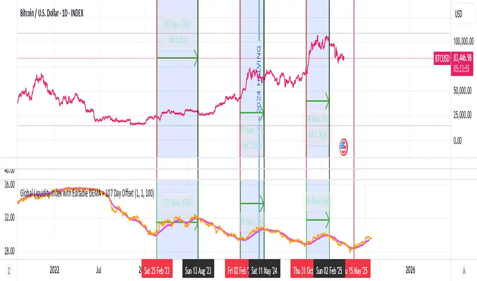
Global Liquidity Index with Editable DEMA + 107 Day OffsetGlobal Liquidity DEMA (107-Day Lead)
This indicator visualizes a smoothed version of global central bank liquidity with a forward time shift of 107 days. The concept is based on the macroeconomic observation that markets tend to lag changes in global liquidity — particularly from central banks like the Federal Reserve, ECB, BOJ, and PBOC.
The script uses a Double Exponential Moving Average (DEMA) to smooth the combined balance sheets and money supply inputs. It then offsets the result into the future by 107 days, allowing you to visually align liquidity trends with delayed market reactions. A second plot (ROC SMA) is included to help identify liquidity momentum shifts.
🔍 How to Use:
Add this indicator to any chart (S&P 500, BTC, Gold, etc.)
Compare price action to the forward-shifted liquidity trend
Look for divergence, confirmation, or crossovers with price
Use as a macro timing tool for long-term entries/exits
📌 Included Features:
Editable DEMA smoothing length
ROC + SMA overlay for momentum signals
Fixed 107-day forward projection
Includes main DEMA and ROC SMA both real-time and shifted
Opal Title: Opal Lines
Short Title: Opal Lines
Description:
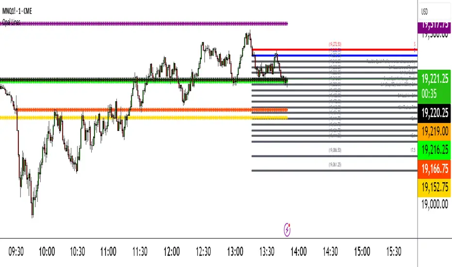
Opal Lines is a dynamic overlay indicator that plots horizontal price levels at the open of key market sessions throughout the trading day, based on Eastern Time (ET). Designed for traders who rely on session-based price action, it marks significant intraday events such as the European Open (3:00 AM ET), Gold Open (8:20 AM ET), Regular Market Open (9:30 AM ET), and Globex Open (6:00 PM ET), among others. Each line is color-coded and toggleable via inputs, allowing users to customize which sessions they want to track.
Unlike generic time-based tools, Opal Lines captures the opening price at precise minute intervals and extends these levels across the chart until the daily reset at 5:00 PM ET (except for the Globex line, which persists into the next day). This makes it ideal for identifying support/resistance zones, breakout levels, or reference points tied to major market openings. Traders can use it across forex, futures, equities, or commodities to align their strategies with global session dynamics.
Key Features:
Seven toggleable session lines with distinct colors for easy identification.
Time-specific logic using ET, adaptable to any chart timeframe.
Persistent lines that reset daily, with Globex extending overnight.
Lightweight and overlay-friendly, preserving chart clarity.
How to Use:
Add the indicator to your chart and enable the sessions relevant to your trading style. Watch for price interactions with these levels—e.g., bounces, breaks, or retests—especially during high-volume periods. Combine with other tools like volume or oscillators for confirmation.
Note: Ensure your chart’s timezone is set to “America/New_York” (ET) for accurate alignment.
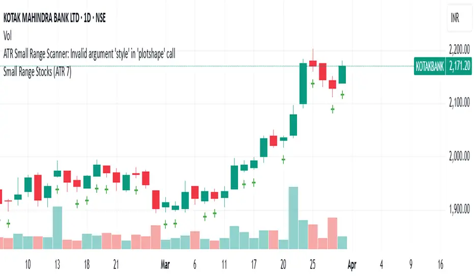
Small Range Stocks (ATR 7)This indicator identifies stocks with a small daily range relative to their ATR(7). It plots a small green tick below candles where the daily range is ≤ 0.9 × ATR(7), helping traders spot consolidation zones for potential breakouts.
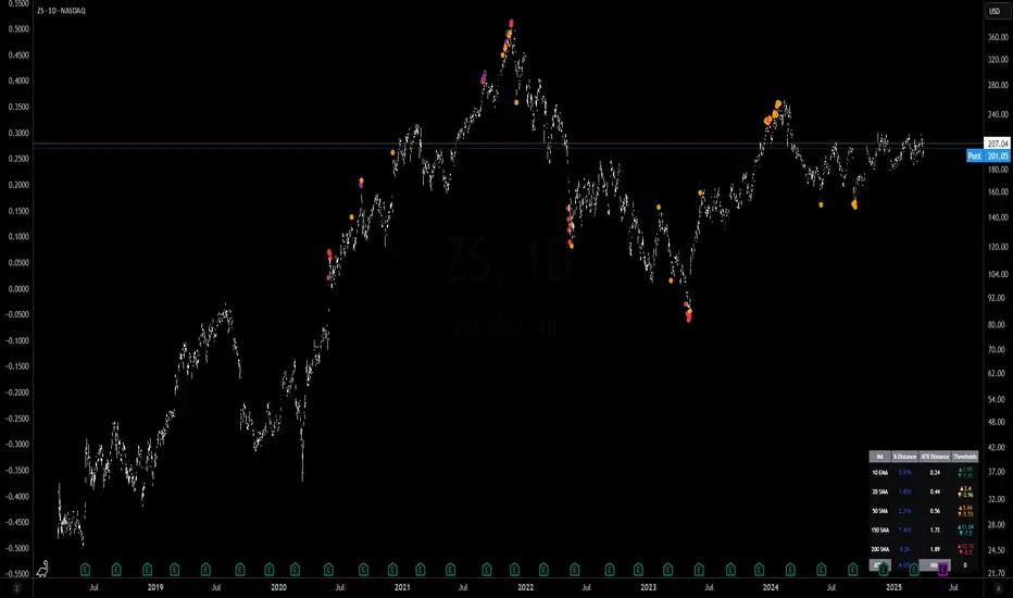
MA Distance (% and ATR) + Threshold CountMA Distance (% & ATR) + Threshold Count
This script visualizes how far price is extended from key moving averages using both percentage and ATR-based distance. It includes a dynamic threshold system that tracks how unusually extended price is, based on historical volatility.
🔍 Features:
Calculates distance from:
10 EMA, 20 SMA, 50 SMA, 100 SMA, 200 SMA
Measures both:
% distance from each MA
ATR-multiple distance from each MA
Automatically calculates dynamic upper/lower thresholds using a rolling standard deviation
Plots a colored dot when distance exceeds these thresholds
Dots appear above or below the bar depending on direction
Color-coded summary table displays:
% distance
ATR distance
Threshold extremes
Total number of threshold hits
🎯 Customization:
Toggle which MAs to display in the table
Set your own lookback window and threshold sensitivity (via stdev multiplier)
Show/hide dots based on how many thresholds are hit
Use this tool to identify when price is overextended from its moving averages and approaching historically significant levels of deviation. Great for spotting mean reversion setups, parabolic runs, or deep pullbacks.
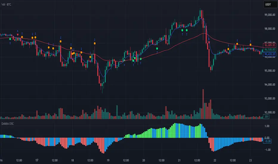
DAMA OSC - Directional Adaptive MA OscillatorOverview:
The DAMA OSC (Directional Adaptive MA Oscillator) is a highly customizable and versatile oscillator that analyzes the delta between two moving averages of your choice. It detects trend progression, regressions, rebound signals, MA cross and critical zone crossovers to provide highly contextual trading information.
Designed for trend-following, reversal timing, and volatility filtering, DAMA OSC adapts to market conditions and highlights actionable signals in real-time.
Features:
Support for 11 custom moving average types (EMA, DEMA, TEMA, ALMA, KAMA, etc.)
Customizable fast & slow MA periods and types
Histogram based on percentage delta between fast and slow MA
Trend direction coloring with “Green”, “Blue”, and “Red” zones
Rebound detection using close or shadow logic
Configurable thresholds: Overbought, Oversold, Underbought, Undersold
Optional filters: rebound validation by candle color or flat-zone filter
Full visual overlay: MA lines, crossover markers, rebound icons
Complete alert system with 16 preconfigured conditions
How It Works:
Histogram Logic:
The histogram measures the percentage difference between the fast and slow MA:
hist_value = ((FastMA - SlowMA) / SlowMA) * 100
Trend State Logic (Green / Blue / Red):
Green_Up = Bullish acceleration
Blue_Up (or Red_Up, depending the display settings) = Bullish deceleration
Blue_Down (or Green_Down, depending the display settings) = Bearish deceleration
Red_Down = Bearish acceleration
Rebound Logic:
A rebound is detected when price:
Crosses back over a selected MA (fast or slow)
After being away for X candles (rebound_backstep)
Optional: filtered by histogram zones or candle color
Inputs:
Display Options:
Show/hide MA lines
Show/hide MA crosses
Show/hide price rebounds
Enable/disable blue deceleration zones
DAMA Settings:
Fast/Slow MA type and length
Source input (close by default)
Overbought/Oversold levels
Underbought/Undersold levels
Rebound Settings:
Use Close and/or Shadow
Rebound MA (Fast/Slow)
Candle color validation
Flat zone filter rebounds (between UnderSold and UnderBought)
Available MA type:
SMA (Simple MA)
EMA (Exponential MA)
DEMA (Double EMA)
TEMA (Triple EMA)
WMA (Weighted MA)
HMA (Hull MA)
VWMA (Volume Weighted MA)
Kijun (Ichimoku Baseline)
ALMA (Arnaud Legoux MA)
KAMA (Kaufman Adaptive MA)
HULLMOD (Modified Hull MA, Same as HMA, tweaked for Pine v6 constraints)
Notes:
**DEMA/TEMA** reduce lag compared to EMA, useful for faster reaction in trending markets.
**KAMA/ALMA** are better suited to noisy or volatile environments (e.g., BTC).
**VWMA** reacts strongly to volume spikes.
**HMA/HULLMOD** are great for visual clarity in fast moves.
Alerts Included (Fully Configurable):
Golden Cross:
Fast MA crosses above Slow MA
Death Cross:
Fast MA crosses below Slow MA
Bullish Rebound:
Rebound from below MA in uptrend
Bearish Rebound:
Rebound from above MA in downtrend
Bull Progression:
Transition into Green_Up with positive delta
Bear Progression:
Transition into Red_Down with negative delta
Bull Regression:
Exit from Red_Down into Blue/Green with negative delta
Bear Regression:
Exit from Green_Up into Blue/Red with positive delta
Crossover Overbought:
Histogram crosses above Overbought
Crossunder Overbought:
Histogram crosses below Overbought
Crossover Oversold:
Histogram crosses above Oversold
Crossunder Oversold:
Histogram crosses below Oversold
Crossover Underbought:
Histogram crosses above Underbought
Crossunder Underbought:
Histogram crosses below Underbought
Crossover Undersold:
Histogram crosses above Undersold
Crossunder Undersold:
Histogram crosses below Undersold
Credits:
Created by Eff_Hash. This code is shared with the TradingView community and full free. do not hesitate to share your best settings and usage.
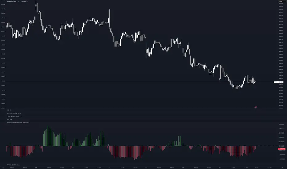
VOLD Ratio Histogram [Th16rry]How to Use the VOLD Ratio Histogram Indicator
The VOLD Ratio Histogram Indicator is a powerful tool for identifying buying and selling volume dominance over a selected period. It provides traders with visual cues about volume pressure in the market, helping them make more informed trading decisions.
How to Read the Indicator:
1. Green Bars (Positive Histogram):
- Indicates that buying volume is stronger than selling volume.
- Higher green bars suggest increasing bullish pressure.
- Useful for confirming uptrends or identifying potential accumulation phases.
2. Red Bars (Negative Histogram):
- Indicates that selling volume is stronger than buying volume.
- Lower red bars suggest increasing bearish pressure.
- Useful for confirming downtrends or identifying potential distribution phases.
3. Zero Line (Gray Line):
- Acts as a neutral reference point where buying and selling volumes are balanced.
- Crossing above zero suggests buying dominance; crossing below zero suggests selling dominance.
How to Use It:
1. Confirming Trends:
- A strong positive histogram during an uptrend supports bullish momentum.
- A strong negative histogram during a downtrend supports bearish momentum.
2. Detecting Reversals:
- Monitor for changes from positive (green) to negative (red) or vice versa as potential reversal signals.
- Divergences between price action and histogram direction can indicate weakening trends.
3. Identifying Volume Surges:
- Sharp spikes in the histogram may indicate strong buying or selling interest.
- Use these spikes to investigate potential breakout or breakdown scenarios.
4. Filtering Noise:
- Adjust the period length to control sensitivity:
- Shorter periods (e.g., 10) are more responsive but may produce more noise.
- Longer periods (e.g., 50) provide smoother signals, better for identifying broader trends.
Recommended Markets:
- Cryptocurrencies: Works effectively with real volume data from exchanges.
- Forex: Useful with tick volume, though interpretation may vary.
- Stocks & Commodities: Particularly effective for analyzing high-volume assets.
Best Practices:
- Combine the VOLD Ratio Histogram with other indicators like moving averages or RSI for confirmation.
- Use different period lengths depending on your trading style (scalping, swing trading, long-term investing).
- Observe volume spikes and divergences to anticipate potential market moves.
The VOLD Ratio Histogram Indicator is ideal for traders looking to enhance their volume analysis and gain a deeper understanding of market dynamics.
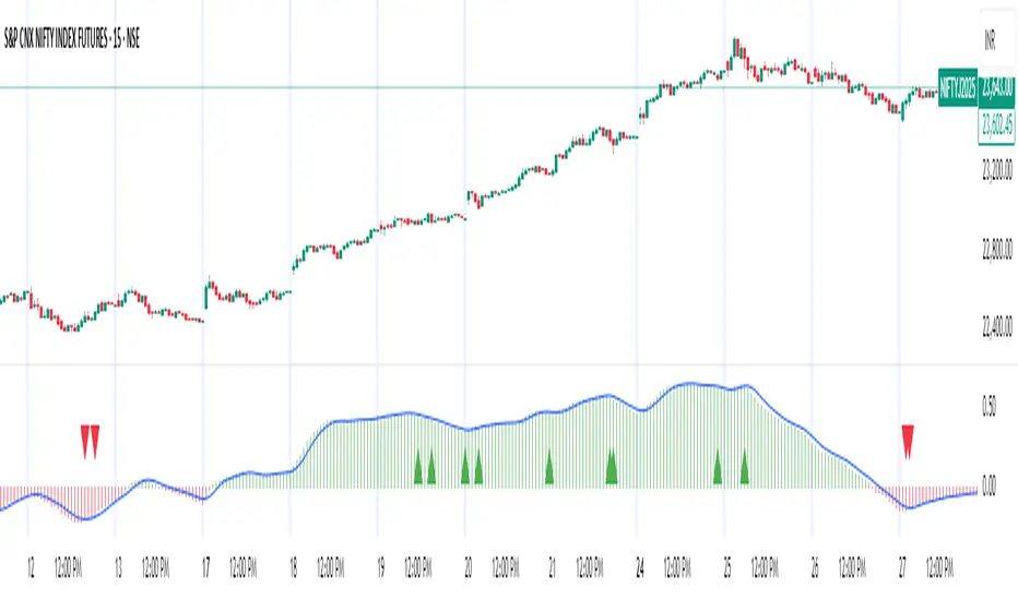
Trend Strength MeterThe Trend Strength Meter (TSM) is a powerful and versatile indicator designed to help traders identify market trends, measure their strength, and detect potential reversals with ease. This indicator combines the power of moving averages, divergence detection, and a clean, customizable dashboard to provide actionable insights for traders of all levels.
How It Works
Trend Strength Calculation:
1. The TSM calculates the trend strength using the difference between two Exponential Moving Averages (EMAs): a fast EMA (default: 20) and a slow EMA (default: 50).
2. The difference is expressed as a percentage of the slow EMA, providing a clear measure of the trend's strength and direction.
Histogram Visualization:
1. A color-coded histogram visually represents the trend strength:
Green: Bullish trend
Red: Bearish trend
Gray: Neutral or no significant trend
2. A smoothed trend strength line (SMA of the trend strength) is also plotted for better clarity.
Divergence Detection:
1. The indicator detects bullish and bearish divergences using the RSI (Relative Strength Index) and price action.
2. Bullish Divergence: Price makes a lower low, but RSI makes a higher low, signaling potential upward momentum.
3. Bearish Divergence: Price makes a higher high, but RSI makes a lower high, signaling potential downward momentum.
=> Divergences are marked with arrows on the chart:
Green Arrow: Bullish divergence
Red Arrow: Bearish divergence
Dashboard:
1. A clean and informative dashboard displays key information:
Trend Strength Value: The current strength of the trend
Trend Direction: Bullish, Bearish, or Neutral
Last Signal: Buy, Sell, or None (based on divergence signals)
The dashboard is fully customizable and can be positioned anywhere on the chart (e.g., top-right, bottom-left, center, etc.).
Key Features
1. Trend Strength Measurement: Quickly identify the strength and direction of the trend.
2. Divergence Detection: Spot potential reversals before they occur with bullish and bearish divergence signals.
3. Customizable Dashboard: Move the dashboard to your preferred location on the chart for better visibility.
4. User-Friendly Design: Clean visuals and intuitive color coding make it easy to interpret market conditions.
5. Actionable Signals: Provides clear Buy/Sell signals based on divergence, helping traders make informed decisions.
How to Use
1. Trend Confirmation:
Use the histogram and trend strength value to confirm the current market trend.
Green bars indicate a bullish trend, while red bars indicate a bearish trend.
2. Divergence Signals:
Look for divergence arrows (green for bullish, red for bearish) to anticipate potential reversals.
Combine divergence signals with other technical analysis tools for higher accuracy.
3. Dashboard Insights:
Monitor the dashboard for real-time updates on trend strength, direction, and the latest signal.
Use the "Last Signal" (Buy/Sell) to validate your trading decisions.
4. Custom Settings:
Adjust the EMA lengths and divergence lookback period to suit your trading style and timeframe.
Position the dashboard anywhere on the chart for convenience.
Best Practices
1. Use the TSM in conjunction with other indicators or price action analysis for confirmation.
2. Test the indicator on different timeframes to find the one that works best for your strategy.
3. Always practice proper risk management when trading.
Disclaimer
This indicator is a tool to assist in technical analysis and should not be used as a standalone trading strategy. Past performance is not indicative of future results. Always conduct your own research and consult with a financial advisor before making trading decisions.
Gold Futures vs Spot (Candlestick + Line Overlay)📝 Script Description: Gold Futures vs Spot
This script was developed to compare the price movements between Gold Futures and Spot Gold within a specific time frame. The primary goals of this script are:
To analyze the price spread between Gold Futures and Spot
To identify potential arbitrage opportunities caused by price discrepancies
To assist in decision-making and enhance the accuracy of gold market analysis
🔧 Key Features:
Fetches price data from both Spot and Futures markets (from APIs or chart sources)
Converts and aligns data for direct comparison
Calculates the price spread (Futures - Spot)
Visualizes the spread over time or exports the data for further analysis
📅 Date Created:
🧠 Additional Notes:
This script is ideal for investors, gold traders, or analysts who want to understand the relationship between the Futures and Spot markets—especially during periods of high volatility. Unusual spreads may signal shifts in market sentiment or the actions of institutional players.

Portfolio Monitor - DolphinTradeBot1️⃣ Overview
▪️This indicator unifies the value of all your investments—whether stocks, currencies, or cryptocurrencies—in your chosen currency. This tool not only provides a clear snapshot of your overall portfolio performance but also highlights the individual growth of each asset with intuitive visualizations and an easy-to-understand performance report.
2️⃣ What sets this indicator apart
▪️is its ability to convert values from various currency pairs into any currency you choose. This means you can monitor your portfolio's performance against any currency pair you prefer, offering a flexible and comprehensive view of your investments.
3️⃣ How Is It Work ?
🔍The indicator can be analyzed under two main categories: visual representations and tables.
1- Visual representations ;
The indicator includes three different types of lines:
1. 1 - Reference Line → This represents the cost of all assets we hold, based on the selected date.
1. 2 - Total Assets Line → Displays the real-time value of all assets in our possession, including cash value, in the selected trading pair.
The area between the reference line is filled with green and red. The section above the reference line is represented in green, while the section below is shown in red.
1. 3 - Performance Lines → These visualize the performance of the assets, starting from the reference line and taking into account their weights in the portfolio. (Note: The lines are scaled for visualization purposes, so their absolute values should not be considered.)
"The names of the lines are shown in the image below."⤵️
2- Tables
The indicator includes three different types of tables:
2. 1 - Analysis Table : It provides a superficial overview of wallet statistics and values.
▪️TOTAL ASSETS → The current equivalent of all assets in the target currency
▪️CASH VALUE → The current value of the amount "Cash Value", in the target currency.
▪️PORTFOLIO VALUE → The total value of assets excluding Cash, in the target currency.
▪️POSTFOLIO COST → The cost of assets excluding Cash, in the target currency.
▪️PORTFOLIO ABSOLUTE RETURN → It shows the profit or loss relative to the cost of assets
▪️PORTFOLIO RETURN % →It shows the profit or loss relative to the cost of assets on a percentage basis
2. 2 - Performance Table : It displays the names of assets excluding Cash and their profit amounts, sorted from highest to lowest profit. If "Show as Percentage" is selected in the settings, it shows the percentage profit or loss relative to the cost. Profits are represented in green, while losses are represented in red.
"You can see the visual showing the tables below"⤵️
4️⃣How to Use ?
1- Choose the date on which the visualization will begin (📌The start date only affects the exchange rate used for calculating the reference line in the target currency.)
2- If you have cash holdings, enter the amount and specify the currency.
3- Select the currency in which your portfolio value will be displayed.(Default value is USD)
4- To set up your portfolio;
SYMBOLS - QUANTITY - PURCHASE PRICE
Enter the symbols of your assets - the number of units you hold - and their cost levels.
5- If you have cash, be sure to include your cash balance. If you also hold other currencies, enter them as separate assets with their corresponding quantities and purchase prices.
6- If you want to see the percentage returns of the assets in the performance table relative to their cost, select the "Show as Percent" option.
7- If you want to see the performance visuals of the assets, click on the "Show Asset Performance" option.
You can find an image of the settings section where the numbers above are used as references below.⤵️
📌 NOTE → By default, a few assets and their values have been pre-added in the initial settings. This is to ensure that you don’t see an empty screen when adding the indicator to the chart. Please remember to enter your own assets and values. The default settings are only provided as an example.

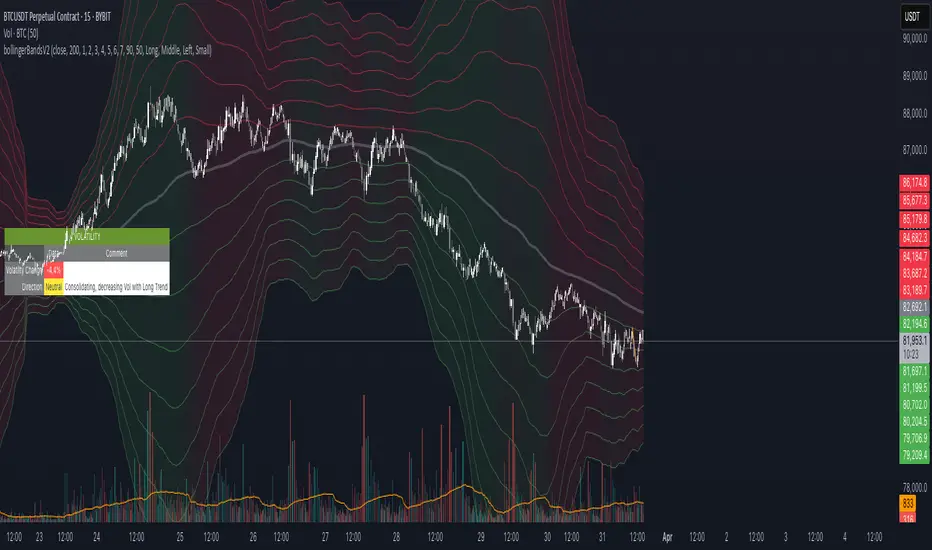
bollingerBandsV2Library "bollingerBandsV2"
Bollinger bands related functions
get_multiple_bollinger_bands(stdv1, stdv2, stdv3, stdv4, stdv5, stdv6, stdv7, length, source)
: Calculates 7 sets of bollinger bands, with 7 different standard deviations
Parameters:
stdv1 (float) : (simple int): standard deviation 1
stdv2 (float) : (simple int): standard deviation 2
stdv3 (float) : (simple int): standard deviation 3
stdv4 (float) : (simple int): standard deviation 4
stdv5 (float) : (simple int): standard deviation 5
stdv6 (float) : (simple int): standard deviation 6
stdv7 (float) : (simple int): standard deviation 7
length (simple int) : (simple int): Length for the bands
source (float) : (simple float): source for the calculation
Returns: : Returns 8 levels plus the range of all the levels.
get_bb_volatility(bb_highest, bb_lowest, ma_length, lookback)
: Provides a volatility indicator based on Bollinger Bands, and indicates wheather the volatility is increasing or decreasing.
Parameters:
bb_highest (float) : (simple float): Top Bollinger Band on which to calculate the range.
bb_lowest (float) : (simple float): Bottom Bollinger Band on which to calculate the range.
ma_length (simple int) : (simple int): Length to use in the smoothing of Bollinger Bands range.
lookback (int) : (simple int): Lookback period to identify a change in the Bollinger Bands range.
Returns: : Returns 8 levels plus the range of all the levels.
get_bbVolatility_data(source, length, stdv1, stdv2, stdv3, stdv4, stdv5, stdv6, stdv7, trend_direction)
: Generates Bollinger Bands Volatility
Parameters:
source (float) : (float): Source for Bollinger Bands
length (simple int) : (int): Length for Bollinger Bands
stdv1 (int) : (int): Standard Deviation 1
stdv2 (int) : (int): Standard Deviation 2
stdv3 (int) : (int): Standard Deviation 3
stdv4 (int) : (int): Standard Deviation 4
stdv5 (int) : (int): Standard Deviation 5
stdv6 (int) : (int): Standard Deviation 6
stdv7 (int) : (int): Standard Deviation 7
trend_direction (string) : (string): Current direction of the trend
Returns: : Returns a map with the levels, plus direction flag and the data table
Linear Regression Volume Profile [ChartPrime]LR VolumeProfile
This indicator combines a Linear Regression channel with a dynamic volume profile, giving traders a powerful way to visualize both directional price movement and volume concentration along the trend.
⯁ KEY FEATURES
Linear Regression Channel: Draws a statistically fitted channel to track the market trend over a defined period.
Volume Profile Overlay: Splits the channel into multiple horizontal levels and calculates volume traded within each level.
Percentage-Based Labels: Displays each level's share of total volume as a percentage, offering a clean way to see high and low volume zones.
Gradient Bars: Profile bars are colored using a gradient scale from yellow (low volume) to red (high volume), making it easy to identify key interest areas.
Adjustable Profile Width and Resolution: Users can change the width of profile bars and spacing between levels.
Channel Direction Indicator: An arrow inside a floating label shows the direction (up or down) of the current linear regression slope.
Level Style Customization: Choose from solid, dashed, or dotted lines for visual preference.
⯁ HOW TO USE
Use the Linear Regression channel to determine the dominant price trend direction.
Analyze the volume bars to spot key levels where the majority of volume was traded—these act as potential support/resistance zones.
Pay attention to the largest profile bars—these often mark zones of institutional interest or price consolidation.
The arrow label helps quickly assess whether the trend is upward or downward.
Combine this tool with price action or momentum indicators to build high-confidence trading setups.
⯁ CONCLUSION
LR Volume Profile is a precision tool for traders who want to merge trend analysis with volume insight. By integrating linear regression trendlines with a clean and readable volume distribution, this indicator helps traders find price levels that matter the most—backed by volume, trend, and structure. Whether you're spotting high-volume nodes or gauging directional flow, this toolkit elevates your decision-making process with clarity and depth.

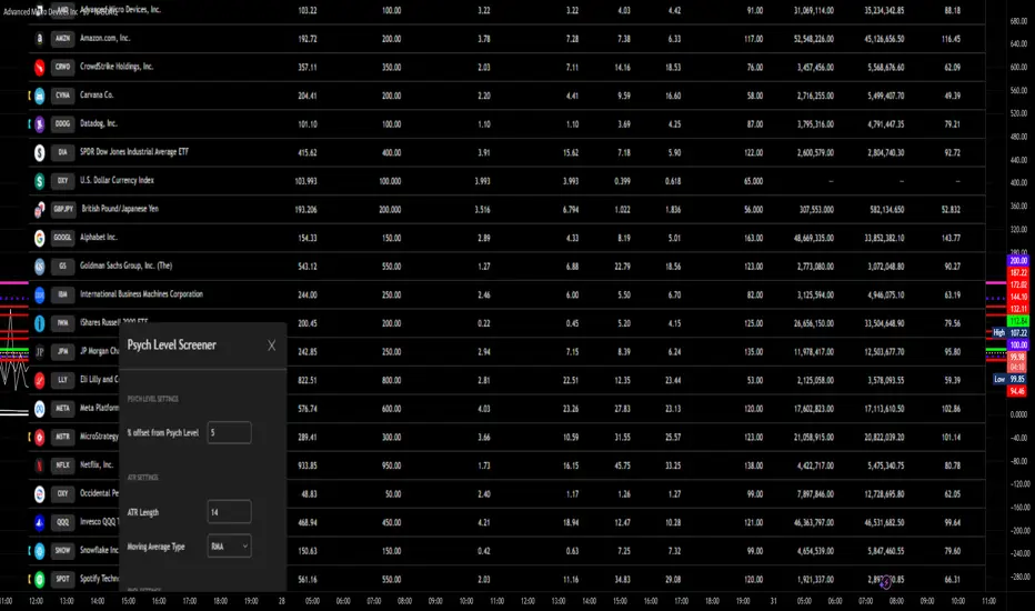
Psych Level ScreenerThis Script is intended for Pine Screener and is not designed as a indicator!!!
Pine Screener is something TradingView has recently added and is still only a Beta version.
Pine Screener itself is currently only available to members that are Premium and above.
What it does:
This screener will actively look for tickers that are close to Pysch level in your watchlist.
Psych level here refers to price levels that are round numbers such as 50,100,1000.
Users can specify the offset from a psych level (in %) and scanner will scan for tickers that are within the offset. For example if offset is set at 5% then it will scan for tickers that are within +/-5% of a ticker. (for $100 psych level it will scan for ticker in $95-105 range)
Once scan is completed you will be able to see:
- Current price of ticker
- Closest psych level for that ticker
- % and $ move required for it to hit that psych level
- Ticker's day range and Average range (with % of average range completed for the day)
- Ticker volume and average volume
Setting up:
www.tradingview.com
Above link will help you guide how to setup Pine screener.
Use steps below to guide you the setup for this specific screener:
1. Open Pine Screener (open new tab, select screener the "Pine")
2. At the top, click on "Choose Indicator" and select "Psych Level Screener"
3. At the top again, click "Indicator Psych Level Screener" and select settings.
4. Change setting to your needs. Hit Apply when done.
a)"% offset from Psych Level" will scan for any stocks in your watchlist which are +/- from the offset you chose for any given psych level. Default is 5. (e.g. If offset is 5%, it will scan for stocks that are between $95-$105 vs $100 psych level, $190-$210 for $200 psych level and so on)
b) ATR length is number of previous trading days you want to include in your calculation. Moving Average Type is calculation method.
c) Rvol length is number of previous trading days you want to include in your calculation.
5. On top left, click "Price within specified offset of Psych. Level" and select true. Then select "Scan" which is located at the top next to "Indicator Psych Level Screener". This will filter out all the stock that meets the condition.
6. At the end of the column on the right there is a "+" symbol. From there you can add/remove columns. 30min/1hr/4hr/1D Trend are disabled by default so if this is needed please enable them.
7. You can change the order of ticker by ascending and descending order of each column label if needed. Just click on the arrow that comes up when you move the cursor to any of the column items.
8. You can specify advanced filter settings based on the variables in the column. (e.g., set price range of stock to filter out further) To do so, click on the column variable name in interest, located above the screener table (or right below "scan") and select "manual setup".
How to read the column:
Current Price: Shows current price of the ticker when scan was done. Currently Pine Screener does NOT support pre/post-hours data so no PM and AH price.
Psych Level: Psych level the current price is near to.
% to Psych Level: Price movement in % necessary to get to the Psych level.
$ to Psych Level: Price movement in $ necessary to get to the Psych level.
DTR: Daily True Range of the stock. i.e. High - Low of the ticker on the day.
ATR: Average True Range of stock in the last x days, where x is a value selected in the setting. (See step 3 in Previous section)
DTR vs ATR: Amount of DTR a ticker has done in % with respect to ATR. (e.g., 90% means DTR is 90% of ATR)
Vol.: Volume of a ticker for the day. Currently Pine Screener does NOT support pre/post-hours data so no PM and AH volume.
Avg. Vol: Average volume of a ticker in the last x days, where x is a value selected in the setting. (See step 3 in Previous section)
Rvol: Relative volume in percentage, measured by the ratio of day's volume and average volume.
30min/1hr/4hr/1D Trend: Trend status to see if the chart is Bullish or Bearish on each of the time frame. Bullishness or Bearishness is defined by the price being over or under the 34/50 cloud on each of the time frame. Output of 1 is Bullish, -1 is Bearish. 0 means price is sitting inside the 34/50 cloud. Currently Pine Screener does NOT support pre/post-hours data so 34/50 cloud is based on regular trading hours data ONLY.
Some things user should be aware of:
- Pine Screener itself is currently only available to TradingView members with Premium Subscription and above. (I can't to anything about this as this is NOT set by me, I have no control) For more info: www.tradingview.com
- The Pine Screener itself is a Beta version and this screener can stop working anytime depending on changes made by TradingView themselves. (Again I cannot control this)
- Pine Screener can only run on Watchlists for now. (as of 03/31/2025) You will have to prepare your own watchlists. In a Watchlist no more than 1000 tickers may be added. (This is TradingView rules)
- Psych level included are currently 50 to 1500 in steps of 50. If you need a specific number please let me know. Will add accordingly.
- Unfortunately this screener does not update automatically, so please hit "scan" to get latest screener result.
- I cannot add 10min trend to the column as Pine Screener does NOT support 10min timeframe as of now. (03/31/2025)
- This code is only meant for Pine Screener. I do NOT recommend using this as an indicator.
- Currently Pine Screener does NOT support pre/post-hours data. So data such as Price, Volume and EMA values are based on market hours data ONLY! (If I'm wrong about this please correct me / let me know and will make look into and make changes to the code)
Other useful links about Pine Screener:
Quick overview of the Screener’s functionality: www.tradingview.com
what do you need to know before you start working? : www.tradingview.com
These links will go over the setting up with GIFs so is easier to understand.
-----------------------------------------------------------------------------------------------------------------
If there are other column variables that you think is worth adding please let me know! Will try add it to the screener!
If you have any questions let me know as well, will reply soon as I can!
Have a good trading day and hope it helps!
Mickey's BBMickey's BB – Smart Reversal Detector with SL Tracking 🔁
This indicator combines the power of Bollinger Bands with engulfing candle patterns to identify high-probability reversal points.
✅ Buy Signal: Triggered when a red candle touches the lower Bollinger Band and is engulfed by a green candle within the next few candles.
✅ Sell Signal: Triggered when a green candle touches the upper Bollinger Band and is engulfed by a red candle within the next few candles.
✅ Smart Lookahead: Scans up to X candles ahead (user-defined) to confirm engulfing reversals — reducing noise in sideways markets.
✅ Dynamic Stop-Loss & Target: Automatically plots SL/TP levels based on user-defined % thresholds.
✅ SL HIT Labels: Highlights exactly when a stop-loss is breached, giving clear visual feedback on trade failures.
✅ Adaptive Market Filter: Signals are only shown when Bollinger Band width exceeds a minimum threshold — filtering out weak/noise signals in low volatility.
🔍 Ideal for reversal traders, scalpers, and those who love combining price action with volatility-based setups.
🛠️ Customizable Parameters:
SMA Period & Std Dev Multiplier (for BB)
SL/Target % levels
Engulf Lookahead range
Minimum BB width to filter signals
🎯 Build it into your strategy, set alerts, or just use it visually to time your entries and exits with clarity.

Momentum Shift [Bigbeluga]
This indicator identifies momentum shifts using a smoothed momentum calculation. It plots dynamic shift zones consisting of five levels that expand or contract based on price action. When momentum rises, the indicator creates an upward shift zone, and when momentum falls, it generates a downward shift zone. The shift zones dynamically react to price, stopping extension when a level is crossed.
🔵Key Features:
Smoothed Momentum Calculation:
➣ Utilizes a Hull Moving Average (HMA) to smooth momentum and reduce noise.
➣ Identifies momentum shifts with crossovers between the current momentum value and its previous state.
➣ Uses a gradient color scheme to highlight momentum strength.
Dynamic Shift Zones:
➣ When momentum rises, the indicator plots an upper shift zone with five incremental levels.
➣ When momentum falls, a lower shift zone is formed with five descending levels.
➣ Each level within the shift zone represents a progressively stronger momentum shift.
Level Extension Control:
➣ Shift zones stop extending once a level is crossed by price.
➣ Levels closer to price act as key momentum resistance or support zones.
➣ If price retraces after a shift, the remaining levels stay intact for further reference.
Momentum Direction Indications:
➣ Labels (▲ and ▼) appear at momentum shift points to indicate rising or falling momentum.
🔵Usage:
Momentum-Based Entries: Identify momentum shifts early by using shift zones as confirmation for trade entries.
Trend Continuation & Exhaustion: Observe which shift levels price respects—if momentum shift zones hold, the trend may continue; if they break, momentum may reverse.
Dynamic Support & Resistance: Use the five-level shift zones as temporary support and resistance areas that adapt to momentum shifts.
Momentum Strength Analysis: If price moves through multiple shift levels in one direction, it signals strong momentum in that direction.
Momentum Shift is a powerful tool for traders looking to analyze momentum shifts with structured visual zones. By combining smoothed momentum calculations with dynamic shift zones, this indicator provides a clear view of market momentum and helps traders navigate price action effectively.

Multi-EMA Crossover StrategyMulti-EMA Crossover Strategy
This strategy uses multiple exponential moving average (EMA) crossovers to identify bullish trends and execute long trades. The approach involves progressively stronger signals as different EMA pairs cross, indicating increasing bullish momentum. Each crossover triggers a long entry, and the intensity of bullish sentiment is reflected in the color of the bars on the chart. Conversely, bearish trends are represented by red bars.
Strategy Logic:
First Long Entry: When the 1-day EMA crosses above the 5-day EMA, it signals initial bullish momentum.
Second Long Entry: When the 3-day EMA crosses above the 10-day EMA, it confirms stronger bullish sentiment.
Third Long Entry: When the 5-day EMA crosses above the 20-day EMA, it indicates further trend strength.
Fourth Long Entry: When the 10-day EMA crosses above the 40-day EMA, it suggests robust long-term bullish momentum.
The bar colors reflect these conditions:
More blue bars indicate stronger bullish sentiment as more short-term EMAs are above their longer-term counterparts.
Red bars represent bearish conditions when short-term EMAs are below longer-term ones.
Example: Bitcoin Trading on a Daily Timeframe
Bullish Scenario:
Imagine Bitcoin is trading at $30,000 on March 31, 2025:
First Signal: The 1-day EMA crosses above the 5-day EMA at $30,000. This suggests initial upward momentum, prompting a small long entry.
Second Signal: A few days later, the 3-day EMA crosses above the 10-day EMA at $31,000. This confirms strengthening bullish sentiment; another long position is added.
Third Signal: The 5-day EMA crosses above the 20-day EMA at $32,500, indicating further upward trend development; a third long entry is executed.
Fourth Signal: Finally, the 10-day EMA crosses above the 40-day EMA at $34,000. This signals robust long-term bullish momentum; a fourth long position is entered.
Bearish Scenario:
Suppose Bitcoin reverses from $34,000 to $28,000:
The 1-day EMA crosses below the 5-day EMA at $33,500.
The 3-day EMA dips below the 10-day EMA at $32,000.
The 5-day EMA falls below the 20-day EMA at $30,000.
The final bearish signal occurs when the 10-day EMA drops below the 40-day EMA at $28,000.
The bars turn increasingly red as bearish conditions strengthen.
Advantages of This Strategy:
Progressive Confirmation: Multiple crossovers provide layered confirmation of trend strength.
Visual Feedback: Bar colors help traders quickly assess market sentiment and adjust positions accordingly.
Flexibility: Suitable for trending markets like Bitcoin during strong rallies or downturns.
Limitations:
Lagging Signals: EMAs are lagging indicators and may react slowly to sudden price changes.
False Breakouts: Crossovers in choppy markets can lead to whipsaws or false signals.
This strategy works best in trending markets and should be combined with additional risk management techniques, e.g., stop loss or optimal position sizes (Kelly Criterion).

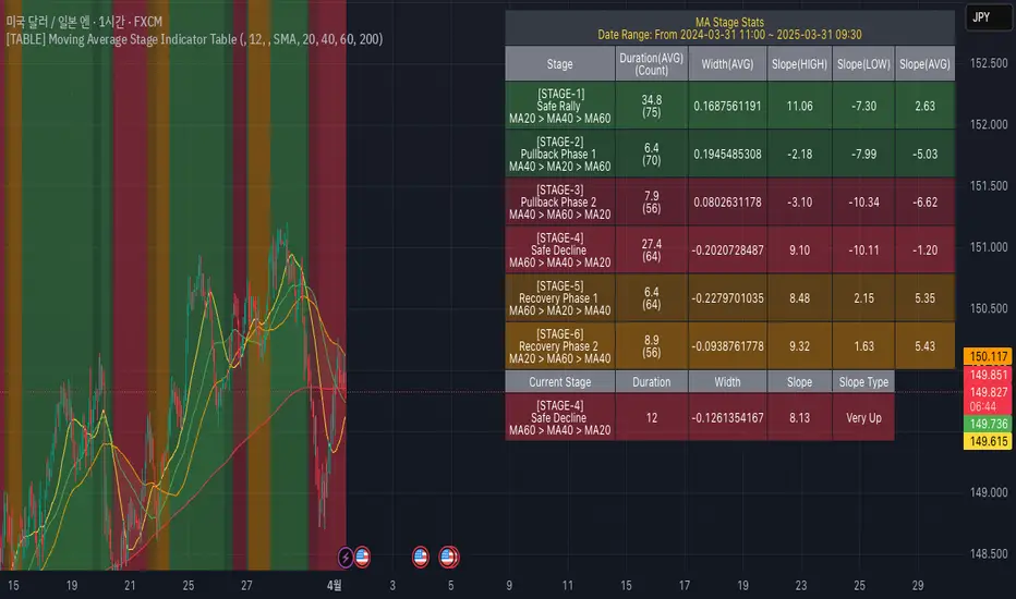
[TABLE] Moving Average Stage Indicator Table📈 MA Stage Indicator Table
🧠 Overview:
This script analyzes market phases based on moving average (MA) crossovers, classifying them into 6 distinct stages and displaying statistical summaries for each.
🔍 Key Features:
• Classifies market condition into Stage 1 to Stage 6 based on the relationship between MA1 (short), MA2 (mid), and MA3 (long)
• Provides detailed stats for each stage:
• Average Duration
• Average Width (MA distance)
• Slope (Angle) - High / Low / Average
• Shows current stage details in real-time
• Supports custom date range filtering
• Choose MA type: SMA or EMA
• Optional background coloring for stages
• Clean summary table displayed on the chart
Adv EMA Cloud v6 (ADX, Alerts)Summary:
This indicator provides a multi-faceted view of market trends using Exponential Moving Averages (EMAs) arranged in visually intuitive clouds, enhanced with an optional ADX-based range filter and configurable alerts for key market conditions. It aims to help traders quickly gauge trend alignment across short, medium, and long timeframes while filtering signals during potentially choppy market conditions.
Key Features:
Multiple EMAs: Displays 10-period (Fast), 20-period (Mid), and 50-period (Slow) EMAs.
Long-Term Trend Filter: Includes a 200-period EMA to provide context for the overall dominant trend direction.
Dual EMA Clouds:
Fast/Mid Cloud (10/20 EMA): Fills the area between the 10 and 20 EMAs. Defaults to Green when 10 > 20 (bullish short-term momentum) and Red when 10 < 20 (bearish short-term momentum).
Mid/Slow Cloud (20/50 EMA): Fills the area between the 20 and 50 EMAs. Defaults to Aqua when 20 > 50 (bullish mid-term trend) and Fuchsia when 20 < 50 (bearish mid-term trend).
Optional ADX Range Filter: Uses the Average Directional Index (ADX) to identify potentially non-trending or choppy markets. When enabled and ADX falls below a user-defined threshold, the EMA clouds will turn grey, visually warning that trend-following signals may be less reliable.
Configurable Alerts: Provides several built-in alert conditions using Pine Script's alertcondition function:
Confluence Condition: Triggers when a 10/20 EMA crossover occurs while both EMA clouds show alignment (both bullish/green/aqua or both bearish/red/fuchsia) and price respects the 200 EMA filter and the ADX filter indicates a trend (if filters are enabled).
MA Filter Cross: Triggers when price crosses above or below the 200 EMA filter line.
Full Alignment Start: Triggers on the first bar where full bullish or bearish alignment occurs (both clouds aligned + MA filter respected + ADX trending, if filters are enabled).
How It Works:
EMA Calculation: Standard Exponential Moving Averages are calculated for the 10, 20, 50, and 200 periods based on the closing price.
Cloud Creation: The fill() function visually shades the area between the 10 & 20 EMAs and the 20 & 50 EMAs.
Cloud Coloring: The color of each cloud is determined by the relationship between the two EMAs that define it (e.g., if EMA 10 is above EMA 20, the first cloud is bullish-colored).
ADX Filter Logic: The script calculates the ADX value. If the "Use ADX Trend Filter?" input is checked and the calculated ADX is below the specified "ADX Trend Threshold", the script considers the market potentially ranging.
ADX Visual Effect: During detected ranging periods (if the ADX filter is active), the plotCloud12Color and plotCloud23Color variables are assigned a neutral grey color instead of their normal bullish/bearish colors before being passed to the fill() function.
Alert Logic: Boolean variables track the specific conditions (crossovers, cloud alignment, filter positions, ADX state). The alertcondition() function creates triggerable alerts based on these pre-defined conditions.
Potential Interpretation (Not Financial Advice):
Trend Alignment: When both clouds share the same directional color (e.g., both bullish - Green & Aqua) and price is on the corresponding side of the 200 EMA filter, it may suggest a stronger, more aligned trend. Conversely, conflicting cloud colors may indicate indecision or transition.
Dynamic Support/Resistance: The EMA lines themselves (especially the 20, 50, and 200) can sometimes act as dynamic levels where price might react.
Range Warning: Greyed-out clouds (when ADX filter is enabled) serve as a visual warning that trend-based strategies might face increased difficulty or whipsaws.
Confluence Alerts: The specific confluence alerts signal moments where multiple conditions align (crossover + cloud agreement + filters), which some traders might view as higher-probability setups.
Customization:
All EMA lengths (10, 20, 50, 200) are adjustable via the Inputs menu.
The ADX length and threshold are configurable.
The MA Trend Filter and ADX Trend Filter can be independently enabled or disabled.
Disclaimer:
This indicator is provided for informational and educational purposes only. Trading financial markets involves significant risk. Past performance is not indicative of future results. Always conduct your own thorough analysis and consider your risk tolerance before making any trading decisions. This indicator should be used in conjunction with other analysis methods and tools. Do not trade based solely on the signals or visuals provided by this indicator.
RSI + MFI Momentum Mapper - CoffeeKillerRSI + MFI Momentum Mapper - CoffeeKiller Indicator Guide
Welcome traders! This guide will walk you through the RSI + MFI Momentum Mapper indicator, an innovative market analysis tool developed by CoffeeKiller that combines two powerful oscillators to create a comprehensive momentum visualization system.
🔔 **Warning: This Is Not a Standard RSI or MFI Indicator** 🔔 This indicator combines and normalizes RSI and MFI data to create a unified momentum representation with boundary detection and peak signaling features.
Core Concept: Combined Momentum Analysis
The foundation of this indicator lies in merging the strengths of two complementary oscillators - Relative Strength Index (RSI) and Money Flow Index (MFI) - to provide a more robust momentum signal that accounts for both price action and volume.
Directional Columns: Momentum Strength
- Positive Green Columns: Bullish momentum
- Negative Red Columns: Bearish momentum
- Color intensity varies based on momentum strength
- Special coloring for new high/low boundaries
Marker Lines: Dynamic Support/Resistance
- High Marker Line (Magenta): Tracks the highest point reached during a bullish phase
- Low Marker Line (Cyan): Tracks the lowest point reached during a bearish phase
- Creates visual boundaries showing momentum extremes
Peak Detection System:
- Triangular markers identify significant local maxima and minima
- Background highlighting shows important momentum peaks
- Helps identify potential reversal points and momentum exhaustion
Reference Lines:
- Zero Line (Gray): Divides bullish from bearish momentum
- High Line (+1): Upper threshold for extremely bullish conditions
- Low Line (-1): Lower threshold for extremely bearish conditions
Core Components
1. Oscillator Normalization
- RSI and MFI values centered around zero
- Values scaled to create consistent visualization
- Normalized range typically between -1 and +1
- Combination of indicators for signal reliability
2. Boundary Tracking System
- Automatic detection of highest values in bullish phases
- Automatic detection of lowest values in bearish phases
- Step-line visualization of boundaries
- Color-coded for easy identification
3. Peak Detection System
- Identification of local maxima and minima
- Background highlighting of significant peaks
- Triangle markers for peak visualization
- Zero-line cross detection for trend changes
4. Signal Smoothing
- Signal line calculation via SMA
- Helps filter noise and identify trends
- Provides confirmation of momentum direction
Main Features
Oscillator Settings
- Customizable RSI length for sensitivity control
- Customizable MFI length for sensitivity control
- Normalized display for consistent visualization
- Signal smoothing for clearer readings
Visual Elements
- Color-coded columns showing momentum direction and strength
- Dynamic marker lines for momentum boundaries
- Peak triangles for significant turning points
- Background highlighting for peak identification
- Reference lines for momentum threshold levels
Signal Generation
- Zero-line crosses for trend change signals
- Boundary breaks for momentum strength
- Peak formation for potential reversals
- Color changes for momentum direction and acceleration
Customization Options
- RSI and MFI length parameters
- Marker line visibility and colors
- Peak marker color selection
- Peak background display options
Trading Applications
1. Trend Identification
- Directional line crossing above zero: bullish trend beginning
- Directional line crossing below zero: bearish trend beginning
- Column color: indicates momentum direction
- Column height: indicates momentum strength
2. Reversal Detection
- Peak triangles after extended trend: potential exhaustion
- Background highlighting: significant reversal points
- Directional line approaching marker lines: potential trend change
- Color shifts from bright to muted: decreasing momentum
3. Momentum Analysis
- Breaking above previous high boundary: accelerating bullish momentum
- Breaking below previous low boundary: accelerating bearish momentum
- Special coloring (magenta/cyan): boundary breaks indicating strength
- Approaching +1/-1 lines: extreme momentum conditions
4. Market Structure Assessment
- Consecutive higher peaks: strengthening bullish structure
- Consecutive lower troughs: strengthening bearish structure
- Peak comparisons: relative strength of momentum phases
- Boundary line steps: market structure levels
Optimization Guide
1. Oscillator Settings
- RSI Length: Default 14 provides balanced signals
- Lower values (7-10): More responsive, potentially noisier
- Higher values (20-30): Smoother, fewer false signals
- MFI Length: Default 14 provides balanced signals
- Lower values: More responsive to volume changes
- Higher values: Less sensitive to short-term volume spikes
2. Visual Customization
- Marker Line Colors: Adjust for visibility on your chart
- Peak Marker Color: Default yellow provides good contrast
- Enable/disable background highlights based on preference
- Consider chart background when selecting colors
3. Signal Interpretation
- Stronger signals: When directional line approaches +1/-1
- Confirmation: When peaks form after extended momentum
- Early warnings: When color intensity changes before direction
- Trend strength: Distance between zero line and current reading
4. Reference Line Usage
- Zero line: Primary trend divider
- +1/-1 lines: Extreme momentum thresholds
- Marker lines: Dynamic support/resistance levels
- Distance from reference: Momentum strength measure
Best Practices
1. Signal Confirmation
- Wait for zero-line crosses to confirm trend changes
- Look for peak formations to identify potential reversals
- Check for boundary breaks to confirm strong momentum
- Use with price action for entry/exit precision
2. Timeframe Selection
- Lower timeframes: more signals, potential noise
- Higher timeframes: cleaner signals, less frequent
- Multiple timeframes: confirm signals across time horizons
- Match to your trading style and holding period
3. Market Context
- Strong bullish phase: positive columns breaking above marker line
- Strong bearish phase: negative columns breaking below marker line
- Columns approaching zero: potential trend change
- Columns approaching +1/-1: extreme conditions, potential reversal
4. Combining with Other Indicators
- Use with trend indicators for confirmation
- Pair with other oscillators for divergence detection
- Combine with volume analysis for validation
- Consider support/resistance levels with boundary lines
Advanced Trading Strategies
1. Boundary Break Strategy
- Enter long when directional line breaks above previous high marker line
- Enter short when directional line breaks below previous low marker line
- Use zero-line as initial stop-loss reference
- Take profits at formation of opposing peaks
2. Peak Trading Strategy
- Identify significant peaks with triangular markers
- Look for consecutive lower peaks in bullish phases for shorting opportunities
- Look for consecutive higher troughs in bearish phases for buying opportunities
- Use zero-line crosses as confirmation
3. Extreme Reading Strategy
- Look for directional line approaching +1/-1 lines
- Watch for color changes and peak formations
- Enter counter-trend positions after confirmed peaks
- Use tight stops due to extreme momentum conditions
4. Column Color Strategy
- Enter long when columns turn bright green (increasing momentum)
- Enter short when columns turn bright red (increasing momentum)
- Exit when color intensity fades (decreasing momentum)
- Use marker lines as dynamic support/resistance
Practical Analysis Examples
Bullish Market Scenario
- Directional line crosses above zero line
- Green columns grow in height and intensity
- High marker line forms steps upward
- Peak triangles appear at local maxima
- Background highlights appear at significant momentum peaks
Bearish Market Scenario
- Directional line crosses below zero line
- Red columns grow in depth and intensity
- Low marker line forms steps downward
- Peak triangles appear at local minima
- Background highlights appear at significant momentum troughs
Consolidation Scenario
- Directional line oscillates around zero line
- Column colors alternate frequently
- Marker lines remain relatively flat
- Few or no new peak highlights appear
- Directional values remain small
Understanding Market Dynamics Through RSI + MFI Momentum Mapper
At its core, this indicator provides a unique lens to visualize market momentum by combining two complementary oscillators:
1. Combined Strength: By averaging RSI (price-based) and MFI (volume-based), the indicator provides a more comprehensive view of market momentum that considers both price action and buying/selling pressure.
2. Normalized Scale: The indicator normalizes values around zero, making it easier to identify bullish vs bearish conditions and the relative strength of momentum in either direction.
3. Dynamic Boundaries: The marker lines create a visual representation of the "high water marks" of momentum in both directions, helping to identify when markets are making new momentum extremes.
4. Exhaustion Signals: The peak detection system highlights moments where momentum has reached a local maximum or minimum, often precursors to reversals or consolidations.
Remember:
- Combine signals from directional line, marker lines, and peak formations
- Use appropriate timeframe settings for your trading style
- Customize the indicator to match your visual preferences
- Consider market conditions and correlate with price action
This indicator works best when:
- Used as part of a comprehensive trading system
- Combined with proper risk management
- Applied with an understanding of current market conditions
- Signals are confirmed by price action and other indicators
DISCLAIMER: This indicator and its signals are intended solely for educational and informational purposes. They do not constitute financial advice. Trading involves significant risk of loss. Always conduct your own analysis and consult with financial professionals before making trading decisions.

02 SMC + BB Breakout (Improved)This strategy combines Smart Money Concepts (SMC) with Bollinger Band breakouts to identify potential trading opportunities. SMC focuses on identifying key price levels and market structure shifts, while Bollinger Bands help pinpoint overbought/oversold conditions and potential breakout points. The strategy also incorporates higher timeframe trend confirmation to filter out trades that go against the prevailing trend.
Key Components:
Bollinger Bands:
Calculated using a Simple Moving Average (SMA) of the closing price and a standard deviation multiplier.
The strategy uses the upper and lower bands to identify potential breakout points.
The SMA (basis) acts as a centerline and potential support/resistance level.
The fill between the upper and lower bands can be toggled by the user.
Higher Timeframe Trend Confirmation:
The strategy allows for optional confirmation of the current trend using a higher timeframe (e.g., daily).
It calculates the SMA of the higher timeframe's closing prices.
A bullish trend is confirmed if the higher timeframe's closing price is above its SMA.
This helps filter out trades that go against the prevailing long-term trend.
Smart Money Concepts (SMC):
Order Blocks:
Simplified as recent price clusters, identified by the highest high and lowest low over a specified lookback period.
These levels are considered potential areas of support or resistance.
Liquidity Zones (Swing Highs/Lows):
Identified by recent swing highs and lows, indicating areas where liquidity may be present.
The Swing highs and lows are calculated based on user defined lookback periods.
Market Structure Shift (MSS):
Identifies potential changes in market structure.
A bullish MSS occurs when the closing price breaks above a previous swing high.
A bearish MSS occurs when the closing price breaks below a previous swing low.
The swing high and low values used for the MSS are calculated based on the user defined swing length.
Entry Conditions:
Long Entry:
The closing price crosses above the upper Bollinger Band.
If higher timeframe confirmation is enabled, the higher timeframe trend must be bullish.
A bullish MSS must have occurred.
Short Entry:
The closing price crosses below the lower Bollinger Band.
If higher timeframe confirmation is enabled, the higher timeframe trend must be bearish.
A bearish MSS must have occurred.
Exit Conditions:
Long Exit:
The closing price crosses below the Bollinger Band basis.
Or the Closing price falls below 99% of the order block low.
Short Exit:
The closing price crosses above the Bollinger Band basis.
Or the closing price rises above 101% of the order block high.
Position Sizing:
The strategy calculates the position size based on a fixed percentage (5%) of the strategy's equity.
This helps manage risk by limiting the potential loss per trade.
Visualizations:
Bollinger Bands (upper, lower, and basis) are plotted on the chart.
SMC elements (order blocks, swing highs/lows) are plotted as lines, with user-adjustable visibility.
Entry and exit signals are plotted as shapes on the chart.
The Bollinger band fill opacity is adjustable by the user.
Trading Logic:
The strategy aims to capitalize on Bollinger Band breakouts that are confirmed by SMC signals and higher timeframe trend. It looks for breakouts that align with potential market structure shifts and key price levels (order blocks, swing highs/lows). The higher timeframe filter helps avoid trades that go against the overall trend.
In essence, the strategy attempts to identify high-probability breakout trades by combining momentum (Bollinger Bands) with structural analysis (SMC) and trend confirmation.
Key User-Adjustable Parameters:
Bollinger Bands Length
Standard Deviation Multiplier
Higher Timeframe
Higher Timeframe Confirmation (on/off)
SMC Elements Visibility (on/off)
Order block lookback length.
Swing lookback length.
Bollinger band fill opacity.
This detailed description should provide a comprehensive understanding of the strategy's logic and components.
***DISCLAIMER: This strategy is for educational purposes only. It is not financial advice. Past performance is not indicative of future results. Use at your own risk. Always perform thorough backtesting and forward testing before using any strategy in live trading.***

Price action plus//The system combines the divergence of A/D and OBV with identifying reversal points using Japanese candlestick patterns, creating an enhanced version of price action. This helps investors more easily and accurately recognize reversal patterns in technical analysis.
Divergence of A/D vs. OBV includes:
Positive divergence: Identifies smart money leaving the market.
Negative divergence: Identifies smart money entering the market.
Reversal candlestick patterns include:
Buy signals: Morning Star, Bullish Engulfing, Hammer.
Strong Buy signals: Buy signals + Negative divergence
Sell signals: Evening Star, Bearish Engulfing, Shooting Star.
Strong Sell signals : Sell signals + Positive divergence
//Hope this system will be helpful for you!

Open Price on Selected TimeframeIndicator Name: Open Price on Selected Timeframe
Short Title: Open Price mtf
Type: Technical Indicator
Description:
Open Price on Selected Timeframe is an indicator that displays the Open price of a specific timeframe on your chart, with the ability to dynamically change the color of the open price line based on the change between the current candle's open and the previous candle's open.
Selectable Timeframes: You can choose the timeframe you wish to monitor the Open price of candles, ranging from M1, M5, M15, H1, H4 to D1, and more.
Dynamic Color Change: The Open price line changes to green when the open price of the current candle is higher than the open price of the previous candle, and to red when the open price of the current candle is lower than the open price of the previous candle. This helps users quickly identify trends and market changes.
Features:
Easy Timeframe Selection: Instead of editing the code, users can select the desired timeframe from the TradingView interface via a dropdown.
Dynamic Color Change: The color of the Open price line changes automatically based on whether the open price of the current candle is higher or lower than the previous candle.
Easily Track Open Price Levels: The indicator plots a horizontal line at the Open price of the selected timeframe, making it easy for users to track this important price level.
How to Use:
Select the Timeframe: Users can choose the timeframe they want to track the Open price of the candles.
Interpret the Color Signal: When the open price of the current candle is higher than the open price of the previous candle, the Open price line is colored green, signaling an uptrend. When the open price of the current candle is lower than the open price of the previous candle, the Open price line turns red, signaling a downtrend.
Observe the Open Price Levels: The indicator will draw a horizontal line at the Open price level of the selected timeframe, allowing users to easily monitor this important price.
Benefits:
Enhanced Technical Analysis: The indicator allows you to quickly identify trends and market changes, making it easier to make trading decisions.
User-Friendly: No need to modify the code; simply select your preferred timeframe to start using the indicator.
Disclaimer:
This indicator is not a complete trading signal. It only provides information about the Open price and related trends. Users should combine it with other technical analysis tools to make more informed trading decisions.
Summary:
Open Price on Selected Timeframe is a simple yet powerful indicator that helps you track the Open price on various timeframes with the ability to change colors dynamically, providing a visual representation of the market's trend.

Pivot Length Percentiles Oscillator# Pivot Length Percentiles Oscillator: Technical Mechanics Explained
## Introduction
The Pivot Length Percentiles Oscillator is a statistical approach to identifying potential market reversals by analyzing the distribution of price movements relative to pivot points. This publication explains the technical mechanics behind the indicator.
## Core Mechanics
### 1. Pivot Point Detection
The indicator begins by identifying significant pivot highs and lows using a user-defined lookback period:
- `lft`: Number of bars to the left of potential pivot point
- `rht`: Number of bars to the right of potential pivot point
These parameters determine how "significant" a pivot needs to be to qualify for analysis.
### 2. Distance Measurement & Historical Database
For each new pivot point identified, the indicator:
- Calculates the absolute price distance from the previous pivot of the same type
- Records the number of candles between consecutive pivots
- Stores these measurements in dynamic arrays that build a historical database
### 3. Statistical Distribution Analysis
Rather than using fixed values, the oscillator analyzes the complete distribution of historical pivot distances and calculates key percentile values:
- `lw` (Low Percentile): Lower boundary for statistical significance
- `md` (Mid Percentile): Median statistical boundary
- `hi` (High Percentile): Upper boundary for statistical extremes
### 4. Oscillator Construction
Two primary oscillator lines are calculated:
- Green line (`osc1`): Measures current price's fall below recent highs with `low - ta.highest(high, lft)`
- Red line (`osc2`): Measures current price's rise above recent lows with `high - ta.lowest(low, lft)`
### 5. Threshold Generation
The percentile values from the historical distribution create dynamic threshold lines:
- For downside movements: Scaled versions of the low percentile (`lw_distance_low`) and high percentile (`hi_distance_low`)
- For upside movements: Scaled versions of the low percentile (`lw_distance_high`) and high percentile (`hi_distance_high`)
### 6. Signal Logic
Entry signals are generated when:
- **Bullish Signal**: The downside oscillator crosses below a statistical threshold while price continues showing downward momentum (close < previous close AND close < previous open)
- **Bearish Signal**: The upside oscillator crosses above a statistical threshold while price continues showing upward momentum (close > previous close AND close > previous open)
### 7. Visualization Options
Users can toggle between:
- Standard view: Shows the oscillator and threshold lines
- Percentile view: Displays the current movement's percentile rank within the historical distribution
## Implementation Notes
- The indicator scales threshold values by 0.9 to create a slight buffer that reduces false signals
- The movement's continuation is confirmed by checking both close-to-close and close-to-open relationships
- Arrays dynamically update throughout the chart's history, making the indicator increasingly accurate as more data is processed
## Mathematical Framework
The core statistical function calculates percentiles using linear interpolation between values when needed:
```
calculate_percentile(array, percentile) =
sortedValue +
fraction * (sortedValue - sortedValue )
```
where `index = (array.size - 1) * percentile / 100`
This mathematical approach ensures the thresholds adapt dynamically to changing market conditions rather than relying on fixed values.