Daily Borders with Weekday Labels[fitfatq]Indicator Overview
This indicator displays daily vertical border lines and the previous day’s weekday label on intraday charts (i.e., charts with a timeframe lower than Daily). It draws a vertical line at the start of each new trading day and places a label displaying the previous day’s weekday (e.g., Monday) at the horizontal midpoint between the previous and the current day. Users can customize various visual aspects such as the separator line style and width, label style, text color, and text size. Additionally, the indicator offers an option to fix the label’s Y coordinate at a specified price level to prevent it from being overlapped by candlesticks.
Parameter Details
Use Fixed Weekday Label Y Coordinate
Type: Boolean
Default: false
Description: When enabled, the weekday label’s vertical position will be fixed at a specified price level (see next parameter). Otherwise, the label’s Y position is determined dynamically (typically based on the current bar’s low minus 3 ticks).
Fixed Weekday Label Y Coordinate (price)
Type: Float
Default: 130.0
Description:
This parameter sets the fixed price level at which the weekday label will be displayed if the "Use Fixed Weekday Label Y Coordinate" option is enabled. Please input a value that corresponds to your chart’s price scale (e.g., 130.50). Note: In charts with high price levels (for example, stocks trading at 3000 or above), it is recommended to set this value to 3000 or above. The higher the value, the closer the label will appear to the candlesticks.
Separator Line Style
Type: String (Options: "Solid", "Dotted", "Dashed")
Default: "Dotted"
Description: Specifies the style of the vertical separator line drawn at the start of each new day. "Solid" displays a continuous line, "Dotted" shows a dotted line, and "Dashed" provides a dashed line.
Separator Line Width
Type: Integer
Default: 1
Description: Determines the thickness of the separator line. A higher number results in a thicker line; the minimum value is 1.
Label Style
Type: String (Options: "None", "Label Up", "Label Down", "Label Left", "Label Right", "Label Center")
Default: "None"
Description: Sets the built-in style for the weekday label. "None" means no background or border (plain text only), while other options apply predefined visual effects.
Text Color
Type: Color
Default: Black
Description: Determines the text color of the weekday label.
Label Text Size
Type: String (Options: "Tiny", "Small", "Normal", "Large", "Huge")
Default: "Normal"
Description: Specifies the text size of the weekday label. Adjust according to preference to ensure the label is readable.
Usage Summary
How It Works:
The indicator detects the start of a new trading day using a change in the daily timeframe (via ta.change(time("D"))). When a new day begins, it draws a vertical separator line at the first bar of that day. If previous day data is available, the indicator calculates the horizontal midpoint between the start of the previous day and the current day and displays the previous day’s weekday label at that position. If the fixed Y coordinate option is enabled, the label is drawn at the specified price level; otherwise, it is positioned relative to the current bar’s low.
Customization:
Users can adjust all visual aspects, including the line style and width as well as the label style, text color, and text size. The fixed Y coordinate option allows the label’s vertical position to remain constant, which helps prevent overlapping with price bars.
Chart Requirement:
This indicator only operates on intraday charts (timeframes lower than Daily) and will not display on Daily or higher timeframe charts.
License
This indicator is released under the Mozilla Public License 2.0. Please credit the original author (fitfatq) when using or sharing this script.
Циклический анализ

Global M2 Money+ Supply Input Lead (USD)Global M2 Money Supply + INR+CAD Input Lead (USD)
This indicator calculates the global M2 money supply in USD by aggregating M2 data from multiple economies, converted to USD using their respective exchange rates. It overlays the scaled M2 data on the chart with a user-defined time shift to analyze potential correlations with asset prices, such as Bitcoin. The indicator is designed to help traders assess global liquidity trends with a customizable lead or lag.
Countries Included:
Eurozone (EUM2)
North America: United States (USM2), Canada (CAM2)
Non-EU Europe: Switzerland (CHM2), United Kingdom (GBM2), Finland (FIM2), Russia (RUM2)
Pacific: New Zealand (NZM2)
Asia: China (CNM2), Taiwan (TWM2), Hong Kong (HKM2), India (INM2), Japan (JPM2), Philippines (PHM2), Singapore (SGM2)
Latin America: Brazil (BRM2), Colombia (COM2), Mexico (MXM2)
Middle East: United Arab Emirates (AEM2), Turkey (TRM2)
Africa: South Africa (ZAM2)
Input for Lead/Lag:
Time Shift (days): Adjust this input to shift the M2 data forward (positive values) or backward (negative values) on the chart. For example, setting a lead of 85 days shifts the M2 data 85 days into the future, helping traders analyze potential leading indicators for price movements.

Webby's Market OrderThis is visual representation of Webby's Market Order.
When three consecutive lows are above 21 EMA, Uptrend expectation is natural.
When three highs are below 21 EMA, Downtrend expectation is natural.
Alert Conditions can be set when uptrend and down trend are expected.
Use this indicator with IXIC or SPY or major indices.
This is set at three lows/Highs above 21 EMA as looked by Mike Webster.

BySq - Market PsychologyThe script I provided is a Market Psychology Index indicator for TradingView, which focuses on three key psychological market phases:
FOMO (Fear of Missing Out)
Panic Selling
Reversal
This indicator uses volume, price changes, and specific time periods to gauge market sentiment. Let me break it down:
1. Input Parameters:
FOMO Period: Defines how many bars (candles) the FOMO index will consider for its calculation.
Panic Period: Defines the period to evaluate Panic Selling.
Reversal Period: Defines the period to evaluate potential price reversals.
You can adjust these periods based on your analysis preferences. The default for each period is 14.
2. FOMO Index:
The FOMO Index aims to capture the "fear of missing out" behavior in the market.
It uses volume and price change:
Volume is compared to the Simple Moving Average (SMA) of volume over the specified period.
Price change is calculated as the percentage change in price compared to the previous bar.
If both volume and price change indicate strong upward movement, the FOMO index spikes.
3. Panic Selling Index:
The Panic Selling Index captures when traders are selling out of fear, often in a rapid or irrational way.
Similar to the FOMO Index, it considers volume and price change:
It uses volume and compares it to the SMA of volume for the panic period.
Price change is negative, meaning it considers only price drops.
When there is high volume coupled with significant price drops, it signals panic selling.
4. Reversal Index:
The Reversal Index aims to detect potential trend reversals in the market.
This index also considers volume and price change:
It focuses on upward price movement and compares volume to its SMA.
If there’s strong upward price movement along with increasing volume, it signals the possibility of a price reversal.
5. Graphical Output:
Histograms are drawn on the chart for each of the three indices:
FOMO is shown in green (indicating the presence of FOMO) and red (when the index is low).
Panic Selling is shown in orange.
Reversal is shown in purple.
The Zero Line (horizontal dotted line) helps identify when any of the indices is positive or negative.
6. Labels:
Labels for each index are shown on the chart at the relevant bar when the index spikes.
FOMO is labeled "FOMO" in green when it spikes.
Panic Selling is labeled "Panic Selling" in orange when it spikes.
Reversal is labeled "Reversal" in purple when it spikes.
Additionally, period labels show above the chart, indicating the specific periods (FOMO, Panic, and Reversal periods) currently being applied. This provides clarity on what time frame each index is analyzing.
7. How to Use:
FOMO: High values may indicate that traders are buying out of fear of missing out on a rally, suggesting a potentially overheated market.
Panic Selling: High values could suggest irrational selling behavior or capitulation, potentially marking the bottom of a downtrend.
Reversal: High values signal the potential for a market reversal, where the price could change direction due to increased volume and upward movement.
8. Visual Appearance:
The indicator’s histograms change colors based on the level of market sentiment detected. The color-coded approach provides an easy-to-read visual representation of different psychological phases in the market.
The horizontal zero line allows easy differentiation between positive and negative values.
Summary:
This script combines the psychology of the market (FOMO, Panic Selling, and Reversal) into a set of indicators that help traders identify potential turning points or emotional states in the market. By focusing on volume and price change, the script attempts to give a clear picture of market sentiment and possible future movements.

SL - 4 EMAs, 2 SMAs & Crossover SignalsThis TradingView Pine Script code is built for day traders, especially those trading crypto on a 1‑hour chart. In simple words, the script does the following:
Calculates Moving Averages:
It computes four exponential moving averages (EMAs) and two simple moving averages (SMAs) based on the closing price (or any price you select). Each moving average uses a different time period that you can adjust.
Plots Them on Your Chart:
The EMAs and SMAs are drawn on your chart in different colors and line thicknesses. This helps you quickly see the short-term and long-term trends.
Generates Buy and Sell Signals:
Buy Signal: When the fastest EMA (for example, a 10-period EMA) crosses above a slightly slower EMA (like a 21-period EMA) and the four EMAs are in a bullish order (meaning the fastest is above the next ones), the script will show a "BUY" label on the chart.
Sell Signal: When the fastest EMA crosses below the second fastest EMA and the four EMAs are lined up in a bearish order (the fastest is below the others), it displays a "SELL" label.
In essence, the code is designed to help you spot potential entry and exit points based on the relationships between multiple moving averages, which work as trend indicators. This makes it easier to decide when to trade on your 1‑hour crypto chart.

StonkGame Major Market Open/ClosePlots vertical lines for Tokyo, London, and New York session opens and closes — auto-adjusted to your chart's timezone.
Open lines = lighter, dashed style.
Close lines = solid, full-color style.
Helps identify key liquidity windows, session-driven volatility, and clean market structure — without chart clutter.
Fully customizable colors and line styles for a professional, minimal look.
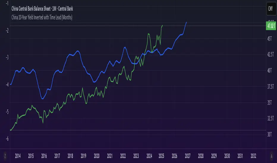
China 10-Year Yield Inverted with Time Lead (Months)The "China 10-Year Yield Inverted with Time Lead (Months)" indicator is a Pine Script tool for TradingView that displays the inverted China 10-Year Government Bond Yield (sourced from TVC:CN10Y) with a user-defined time lead or lag in months. The yield is inverted by multiplying it by -1, making a rising yield appear as a downward movement and vice versa, which helps visualize inverse correlations with other assets. Users can input the number of months to shift the yield forward (lead) or backward (lag), with the shift calculated based on the chart’s timeframe (e.g., 20 bars per month on daily charts). The indicator plots the shifted, inverted yield as a blue line in a separate pane, with a zero line for reference, enabling traders to analyze leading or lagging relationships with other financial data, such as the PBOC Balance Sheet or Bitcoin price.
Price Position Percentile (PPP)
Price Position Percentile (PPP)
A statistical analysis tool that dynamically measures where current price stands within its historical distribution. Unlike traditional oscillators, PPP adapts to market conditions by calculating percentile ranks, creating a self-adjusting framework for identifying extremes.
How It Works
This indicator analyzes the last 200 price bars (customizable) and calculates the percentile rank of the current price within this distribution. For example, if the current price is at the 80th percentile, it means the price is higher than 80% of all prices in the lookback period.
The indicator creates five dynamic zones based on percentile thresholds:
Extremely Low Zone (<5%) : Prices in the lowest 5% of the distribution, indicating potential oversold conditions.
Low Zone (5-25%) : Accumulation zone where prices are historically low but not extreme.
Neutral Zone (25-75%) : Fair value zone representing the middle 50% of the price distribution.
High Zone (75-95%) : Distribution zone where prices are historically high but not extreme.
Extremely High Zone (>95%) : Prices in the highest 5% of the distribution, suggesting potential bubble conditions.
Mathematical Foundation
Unlike fixed-threshold indicators, PPP uses a non-parametric approach:
// Core percentile calculation
percentile = (count_of_prices_below_current / total_prices) * 100
// Threshold calculation using built-in function
p_extremely_low = ta.percentile_linear_interpolation(source, lookback, 5)
p_low = ta.percentile_linear_interpolation(source, lookback, 25)
p_neutral_high = ta.percentile_linear_interpolation(source, lookback, 75)
p_extremely_high = ta.percentile_linear_interpolation(source, lookback, 95)
Key Features
Dynamic Adaptation : All zones adjust automatically as price distribution changes
Statistical Robustness : Works on any timeframe and any market, including highly volatile cryptocurrencies
Visual Clarity : Color-coded zones provide immediate visual context
Non-parametric Analysis : Makes no assumptions about price distribution shape
Historical Context : Shows how zones evolved over time, revealing market regime changes
Practical Applications
PPP provides objective statistical context for price action, helping traders make more informed decisions based on historical price distribution rather than arbitrary levels.
Value Investment : Identify statistically significant low prices for potential entry points
Risk Management : Recognize when prices reach historical extremes for profit taking
Cycle Analysis : Observe how percentile zones expand and contract during different market phases
Market Regime Detection : Identify transitions between accumulation, markup, distribution, and markdown phases
Usage Guidelines
This indicator is particularly effective when:
- Used across multiple timeframes for confirmation
- Combined with volume analysis for validation of extremes
- Applied in conjunction with trend identification tools
- Monitored for divergences between price action and percentile ranking

Vwap Vision #WhiteRabbitVWAP Vision #WhiteRabbit
This Pine Script (version 5) script implements a comprehensive trading indicator called "VWAP Vision #WhiteRabbit," designed for analyzing price movements using the Volume-Weighted Average Price (VWAP) along with multiple customizable features, including adjustable color themes for better visual appeal.
Features:
Customizable Color Themes:
Choose from four distinct themes: Classic, Dark Mode, Fluo, and Phil, enhancing the visual layout to match user preferences.
VWAP Calculation:
Uses standard VWAP calculations based on selected anchor periods (Session, Week, Month, etc.) to help identify price trends.
Band Settings:
Multiple bands are calculated based on standard deviations or percentages, with customization options to configure buy/sell zones and liquidity levels.
Buy/Sell Signals:
Generates clear buy and sell signals based on price interactions with the calculated bands and the exponential moving average (EMA).
Real-time Data Display:
Displays real-time signals and VWAP values for selected trading instruments, including XAUUSD, NAS100, and BTCUSDT, along with related alerts for trading opportunities.
Volatility Analysis:
Incorporates volatility metrics using the Average True Range (ATR) to assess market conditions and inform trading decisions.
Enhanced Table Displays:
Provides tables for clear visualization of trading signals, real-time data, and performance metrics.
This script is perfect for traders looking to enhance their analysis and gain insights for making informed trading decisions across various market conditions.

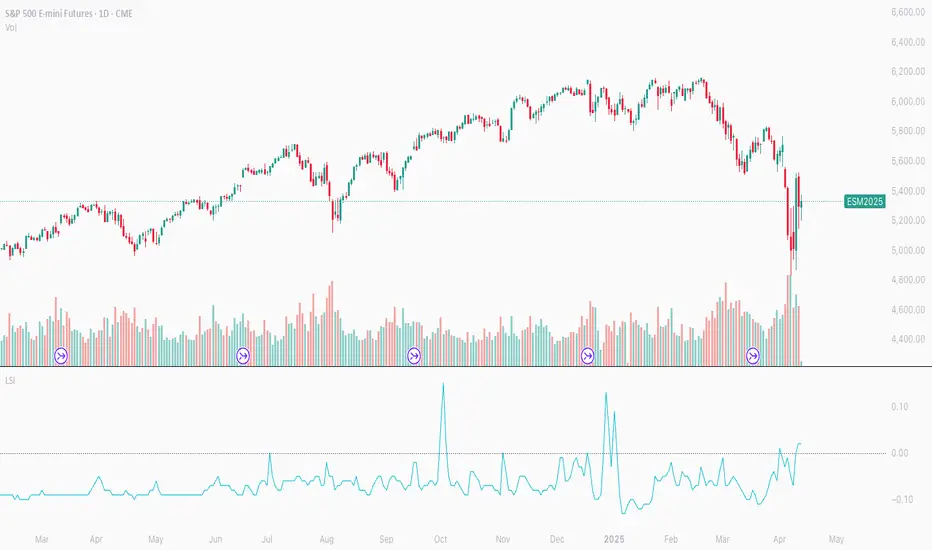
Liquidity Stress Index SOFR - IORBLiquidity Stress Index (SOFR - IORB)
This indicator tracks the spread between the Secured Overnight Financing Rate (SOFR) and the Interest on Reserve Balances (IORB) set by the Federal Reserve.
A persistently positive spread may indicate funding stress or liquidity shortages in the repo market, as it suggests overnight lending rates exceed the risk-free rate banks earn at the Fed.
Useful for monitoring monetary policy transmission or market/liquidity stress.
Quarterly Cycle Theory with DST time AdjustedThe Quarterly Theory removes ambiguity, as it gives specific time-based reference points to look for when entering trades. Before being able to apply this theory to trading, one must first understand that time is fractal:
Yearly Quarters = 4 quarters of three months each.
Monthly Quarters = 4 quarters of one week each.
Weekly Quarters = 4 quarters of one day each (Monday - Thursday). Friday has its own specific function.
Daily Quarters = 4 quarters of 6 hours each = 4 trading sessions of a trading day.
Sessions Quarters = 4 quarters of 90 minutes each.
90 Minute Quarters = 4 quarters of 22.5 minutes each.
Yearly Cycle: Analogously to financial quarters, the year is divided in four sections of three months each:
Q1 - January, February, March.
Q2 - April, May, June (True Open, April Open).
Q3 - July, August, September.
Q4 - October, November, December.
S&P 500 E-mini Futures (daily candles) — Monthly Cycle.
Monthly Cycle: Considering that we have four weeks in a month, we start the cycle on the first month’s Monday (regardless of the calendar Day):
Q1 - Week 1: first Monday of the month.
Q2 - Week 2: second Monday of the month (True Open, Daily Candle Open Price).
Q3 - Week 3: third Monday of the month.
Q4 - Week 4: fourth Monday of the month.
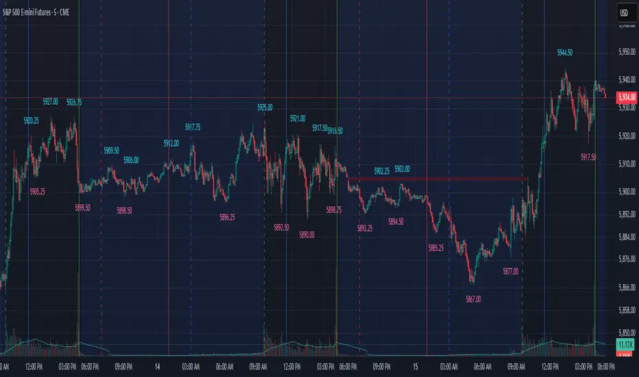
S&P 500 E-mini Futures (4 hour candles) — Weekly Cycle.
Weekly Cycle: Daye determined that although the trading week is composed by 5 trading days, we should ignore Friday, and the small portion of Sunday’s price action:
Q1 - Monday.
Q2 - Tuesday (True Open, Daily Candle Open Price).
Q3 - Wednesday.
Q4 - Thursday.
S&P 500 E-mini Futures (1 hour candles) — Daily Cycle.
Daily Cycle: The Day can be broken down into 6 hour quarters. These times roughly define the sessions of the trading day, reinforcing the theory’s validity:
Q1 - 18:00 - 00:00 Asia.
Q2 - 00:00 - 06:00 London (True Open).
Q3 - 06:00 - 12:00 NY AM.
Q4 - 12:00 - 18:00 NY PM.
S&P 500 E-mini Futures (15 minute candles) — 6 Hour Cycle.
6 Hour Quarters or 90 Minute Cycle / Sessions divided into four sections of 90 minutes each (EST/EDT):
Asian Session
Q1 - 18:00 - 19:30
Q2 - 19:30 - 21:00 (True Open)
Q3 - 21:00 - 22:30
Q4 - 22:30 - 00:00
London Session
Q1 - 00:00 - 01:30
Q2 - 01:30 - 03:00 (True Open)
Q3 - 03:00 - 04:30
Q4 - 04:30 - 06:00
NY AM Session
Q1 - 06:00 - 07:30
Q2 - 07:30 - 09:00 (True Open)
Q3 - 09:00 - 10:30
Q4 - 10:30 - 12:00
NY PM Session
Q1 - 12:00 - 13:30
Q2 - 13:30 - 15:00 (True Open)
Q3 - 15:00 - 16:30
Q4 - 16:30 - 18:00
S&P 500 E-mini Futures (5 minute candles) — 90 Minute Cycle.
Micro Cycles: Dividing the 90 Minute Cycle yields 22.5 Minute Quarters, also known as Micro Sessions or Micro Quarters:
Asian Session
Q1/1 18:00:00 - 18:22:30
Q2 18:22:30 - 18:45:00
Q3 18:45:00 - 19:07:30
Q4 19:07:30 - 19:30:00
Q2/1 19:30:00 - 19:52:30 (True Session Open)
Q2/2 19:52:30 - 20:15:00
Q2/3 20:15:00 - 20:37:30
Q2/4 20:37:30 - 21:00:00
Q3/1 21:00:00 - 21:23:30
etc. 21:23:30 - 21:45:00
London Session
00:00:00 - 00:22:30 (True Daily Open)
00:22:30 - 00:45:00
00:45:00 - 01:07:30
01:07:30 - 01:30:00
01:30:00 - 01:52:30 (True Session Open)
01:52:30 - 02:15:00
02:15:00 - 02:37:30
02:37:30 - 03:00:00
03:00:00 - 03:22:30
03:22:30 - 03:45:00
03:45:00 - 04:07:30
04:07:30 - 04:30:00
04:30:00 - 04:52:30
04:52:30 - 05:15:00
05:15:00 - 05:37:30
05:37:30 - 06:00:00
New York AM Session
06:00:00 - 06:22:30
06:22:30 - 06:45:00
06:45:00 - 07:07:30
07:07:30 - 07:30:00
07:30:00 - 07:52:30 (True Session Open)
07:52:30 - 08:15:00
08:15:00 - 08:37:30
08:37:30 - 09:00:00
09:00:00 - 09:22:30
09:22:30 - 09:45:00
09:45:00 - 10:07:30
10:07:30 - 10:30:00
10:30:00 - 10:52:30
10:52:30 - 11:15:00
11:15:00 - 11:37:30
11:37:30 - 12:00:00
New York PM Session
12:00:00 - 12:22:30
12:22:30 - 12:45:00
12:45:00 - 13:07:30
13:07:30 - 13:30:00
13:30:00 - 13:52:30 (True Session Open)
13:52:30 - 14:15:00
14:15:00 - 14:37:30
14:37:30 - 15:00:00
15:00:00 - 15:22:30
15:22:30 - 15:45:00
15:45:00 - 15:37:30
15:37:30 - 16:00:00
16:00:00 - 16:22:30
16:22:30 - 16:45:00
16:45:00 - 17:07:30
17:07:30 - 18:00:00
S&P 500 E-mini Futures (30 second candles) — 22.5 Minute Cycle.

Filtered Swing Pivot S&R )Pivot support and resis🔍 Filtered Swing Pivot S&R - Overview
This indicator identifies and plots tested support and resistance levels using a filtered swing pivot strategy. It focuses on high-probability zones where price has reacted before, helping traders better anticipate future price behavior.
It filters out noise using:
Customizable pivot detection logic
Minimum price level difference
ATR (Average True Range) volatility filter
Confirmation by price retesting the level before plotting
⚙️ Core Logic Explained
✅ 1. Pivot Detection
The script uses Pine Script's built-in ta.pivothigh() and ta.pivotlow() functions to find local highs (potential resistance) and lows (potential support).
Pivot Lookback/Lookahead (pivotLen):
A pivot is confirmed if it's the highest (or lowest) point within a lookback and lookahead range of pivotLen bars.
Higher values = fewer, stronger pivots.
Lower values = more, but potentially noisier levels.
✅ 2. Pending Pivot Confirmation
Once a pivot is detected:
It is not drawn immediately.
The script waits until price re-tests that pivot level. This retest confirms the market "respects" the level.
For example: if price hits a previous high again, it's treated as a valid resistance.
✅ 3. Dual-Level Filtering System
To reduce chart clutter and ignore insignificant levels, two filters are applied:
Fixed Threshold (Minimum Level Difference):
Ensures a new pivot level is not too close to the last one.
ATR-Based Filter:
Dynamically adjusts sensitivity based on current volatility using the formula:
java
Copy
Edit
Minimum distance = ATR × ATR Multiplier
Only pivots that pass both filters are plotted.
✅ 4. Line Drawing
Once a pivot is:
Detected
Retested
Filtered
…a horizontal dashed line is drawn at that level to highlight support or resistance.
Resistance: Red (default)
Support: Green (default)
These lines are:
Dashed for clarity
Extended for X bars into the future (user-defined) for forward visibility
🎛️ Customizable Inputs
Parameter Description
Pivot Lookback/Lookahead Bars to the left and right of a pivot to confirm it
Minimum Level Difference Minimum price difference required between plotted levels
ATR Length Number of bars used in ATR volatility calculation
ATR Multiplier for Pivot Multiplies ATR to determine volatility-based pivot separation
Line Extension (bars) How many future bars the level line will extend for better visibility
Resistance Line Color Color for resistance lines (default: red)
Support Line Color Color for support lines (default: green)
📈 How to Use It
This indicator is ideal for:
Identifying dynamic support & resistance zones that adapt to volatility.
Avoiding false levels by waiting for pivot confirmation.
Visual guidance for entries, exits, stop placements, or take-profits.
🔑 Trade Ideas:
Use support/resistance retests for entry confirmations.
Combine with candlestick patterns or volume spikes near drawn levels.
Use in confluence with trendlines or moving averages.
🚫 What It Does Not Do (By Design)
Does not repaint or remove past levels once confirmed.
Does not include labels or alerts (but can be added).
Does not auto-scale based on timeframes (manual tuning recommended).
🛠️ Possible Enhancements (Optional)
If desired, you could extend the functionality to include:
Labels with “S” / “R”
Alert when a new level is tested or broken
Toggle for support/resistance visibility
Adjustable line width or style
tance indicator

Stoch_RSIStochastic RSI – Advanced Divergence Indicator
This custom indicator is an advanced version of the Stochastic RSI that not only smooths and refines the classic RSI input but also automatically detects both regular and hidden divergences using two powerful methods: fractal-based and pivot-based detection. Originally inspired by contributions from @fskrypt, @RicardoSantos, and later improved by developers like @NeoButane and @FYMD, this script has been fully refined for clarity and ease-of-use.
Key Features:
Dual Divergence Detection:
Fractal-Based Divergence: Uses a four-candle pattern to confirm top and bottom fractals for bullish and bearish divergences.
Pivot-Based Divergence: Employs TradingView’s built-in pivot functions for an alternate view of divergence conditions.
Customizable Settings:
The inputs are organized into logical groups (Stoch RSI settings, Divergence Options, Labels, and Market Open Settings) allowing you to adjust smoothing periods, RSI and Stochastic lengths, and divergence thresholds with a user-friendly interface.
Visual Enhancements:
Plots & Fills: The indicator plots both the K and D lines with corresponding fills and horizontal bands for quick visual reference.
Divergence Markers: Diamond shapes and labeled markers indicate regular and hidden divergences on the chart.
Market Open Highlighting: Optional histogram plots highlight the market open candle based on different timeframes for stocks versus non-forex symbols.

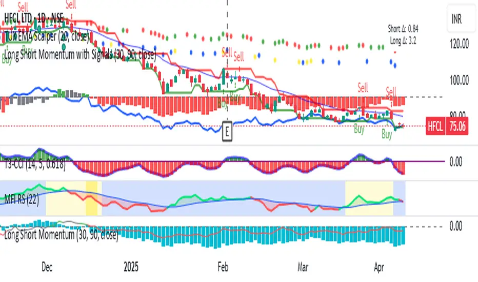
Long Short Momentum with Signals
Long and Short momentum
WHEN SHORT MOMENTUM CHANGES 2.0 POINTS and long term changes 5 points on day basis write A for Bullish and B for Bearish on Main Price chart
WHEN SHORT MOMENTUM CHANGES .30 per hour POINTS and long term changes 1 points on 1 hour basis. Put a green dot for Bull and red for bear in short term and for long termRespectively on price chart
PMO + Daily SMA(55)PMO + Daily SMA(55)
This script plots the Price Momentum Oscillator (PMO) using the classic DecisionPoint methodology, along with its signal line and the 55-period Simple Moving Average (SMA) of the daily PMO.
PMO is a smoothed momentum indicator that measures the rate of change and helps identify trend direction and strength. The signal line is an EMA of the PMO, commonly used for crossover signals.
The 55-period SMA of the daily PMO is added as a longer-term trend filter. It remains based on daily data, even when applied to intraday charts, making it useful for aligning lower timeframe trades with higher timeframe momentum.
Ideal for swing and position traders looking to combine short-term momentum with broader trend context.

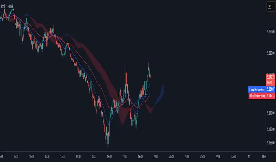
TCloud Future📘 Tcloud Future – Indicator Description & How to Use
Tcloud Future is a trend-based indicator that creates a forward-projected cloud between:
A customizable Exponential Moving Average (EMA)
A dynamic McGinley Moving Average
The cloud is shifted into the future (like the Ichimoku Cloud), giving traders a visual projection of potential trend direction.
🔧 Components:
EMA (default: 19-period) – fast-reacting average to short-term price action
McGinley Dynamic (default: 26-period) – smoother, adaptive average that reacts to volatility
Forward Projection (default: 26 candles) – pushes the cloud into the future to help anticipate trend continuation or reversal
Cloud Color
Green when EMA is above McGinley (bullish bias)
Red when EMA is below McGinley (bearish bias)
🟢 How to Trade with Tcloud Future
✅ Trend Confirmation
Use the cloud color and slope to confirm the current trend.
Green cloud sloping up → bullish momentum
Red cloud sloping down → bearish momentum
🟩 Entry Strategy (Trend-Following)
Go long when price is above the green cloud and the cloud is rising.
Go short when price is below the red cloud and the cloud is falling.
🔁 Cloud Crossovers (Trend Shift)
A color change in the projected cloud can signal a potential trend reversal.
Use this as a heads-up to prepare for position changes or tighten stops.
🛡️ Support/Resistance Zones
The cloud often acts as a dynamic support/resistance zone.
During an uptrend, pullbacks to the top or middle of the green cloud can be good entries.
During a downtrend, rallies into the red cloud can offer shorting opportunities.
🧠 Tips
Combine with RSI, MACD, or Volume for confirmation.
Avoid using it alone in sideways markets — it performs best in trending conditions.
Adjust projection and smoothing settings to fit the asset/timeframe you're trading.
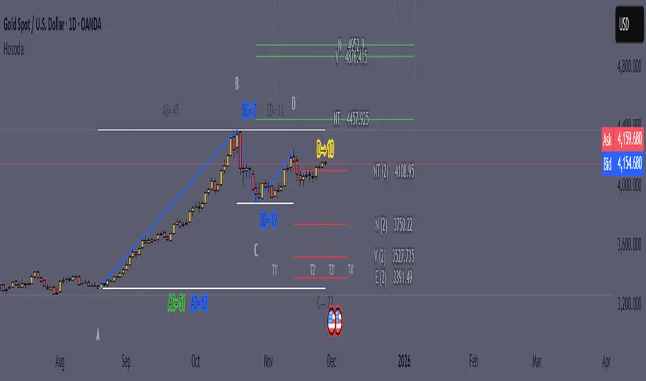
Goichi Hosoda TheoryGreetings to traders. I offer you an indicator for trading according to the Ichimoku Kinho Hyo trading system. This indicator determines possible time cycles of price reversal and expected asset price values based on the theory of waves and time cycles by Goichi Hosoda.
The indicator contains classic price levels N, V, E and NT, and is supplemented with intermediate levels V+E, V+N, N+NT and x2, x3, x4 for levels V and E, which are used in cases where the wave does not contain corrections and there is no possibility to update the impulse-corrective wave.
A function for counting bars from points A B and C has also been added.
Larsson Line Replica (Yellow = Bullish, Blue = Bearish)📘 Interpretation with Flipped Colors
🟨 Yellow Zones – Bullish Trend
• Signals uptrend confirmation.
• SMMA(15) > SMMA(29) indicates upward momentum.
• Ideal for:
• Holding or adding to long positions
• Buying pullbacks within or near the band
• Ignoring short setups on lower timeframes unless reversal signals show up
🟦 Blue Zones – Bearish Trend
• SMMA(15) < SMMA(29) confirms a downtrend.
• Useful for:
• Risk-off posture: take profits, reduce exposure
• Considering short trades
• Waiting out until trend flips yellow again before longing
🩶 Gray Zones – Transition / Unclear
• Represents possible trend change or indecision.
• Appears around crossovers.
• Great time to be cautious — wait for confirmation (either yellow or blue)
• Often coincides with low-volatility consolidation zones or false breakouts
📊 Timeframe Interpretation Tips (with Updated Colors)
🕰️ Weekly – Macro Regime Filter
• 🟨 Yellow = Swing longs allowed
• 🟦 Blue = Risk-off, short setups more reliable
• Use this timeframe as your macro bias anchor
• Combine with higher timeframe market structure, moving averages, or on-chain trends
⸻
📅 Daily – Tactical Entry & Position Management
• Use the slope of the bands for early momentum detection
• 🟦 Blue to Yellow flips = potential trend reversal to the upside → re-enter longs, cut shorts
• 🟨 Yellow to Blue flips = trend weakness or downtrend return → consider profit-taking or short setups
• Great timeframe for:
• Refining entries
• Managing exits
• Spotting trend shifts before weekly confirms
⸻
⏱ Lower Timeframes (4H, 1H) – Execution
• Treat the band like a dynamic trend channel
• Enter trades in direction of the current color:
• 🟨 Yellow → Buy pullbacks to the midline
• 🟦 Blue → Sell bounces into the midline
• Avoid trading against the band unless clear structure or divergence forms
• Pair with RSI/MACD for confluence

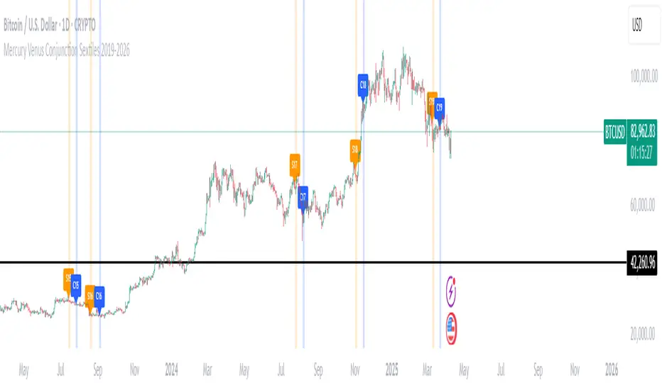
Mercury Venus Conjunction Sextiles 2019-2026How to Use It and What It Means Astrologically
How to Use the Script in TradingView
This Pine Script, called "Mercury Venus Aspects 2019–2026," is made to highlight the dates of Mercury-Venus conjunctions (0°) and sextiles (60°) from 2019 to 2026 on TradingView charts. Here's how to use it:
click “Add to Chart.” It will apply to any chart you have open—stocks, forex, crypto, etc.
Customize the Display
You can turn on/off the visibility of conjunctions and sextiles using checkboxes under "Inputs" in the settings.
You can also adjust the label size (small, normal, large, or huge) for better readability on your chart.
What You’ll See on the Chart
Conjunctions appear as blue shaded zones with labels like “C1,” “C2,” etc. These mark dates when Mercury and Venus are at the same degree.
Sextiles show up in orange with labels like “S1,” “S2,” marking when they’re about 60° apart.
Each event spans a 2-day window (one day before and after the exact aspect).
How to Use It Practically
You can overlay the script on market charts to look for any patterns between these planetary aspects and price movements.
You can also use it to plan personal or financial activities, since these aspects often affect communication, money, and relationships.
What to Keep in Mind
Dates are approximate and based on average planetary cycles (Mercury: ~88 days, Venus: ~225 days). For exact timing, use an ephemeris.
Only conjunctions and sextiles are shown. Oppositions, squares, and trines aren’t included because Mercury and Venus never get far enough apart (more than 75°).
This script is great for astrologers, traders, and enthusiasts who want to see Mercury-Venus aspects directly on their charts and explore their possible effects.
Astrological Meaning of Mercury-Venus Aspects
What Mercury and Venus Represent
Mercury rules communication, thinking, technology, travel, and trade. In global events (mundane astrology), it affects media, markets, and movement of information.
Venus is about love, beauty, money, and pleasure. It influences relationships, aesthetics, and finance. In the world stage, it’s linked to luxury, art, fashion, and economic balance.
When Mercury and Venus form aspects (like conjunctions or sextiles), their energies mix in helpful ways that can affect people and events.
Conjunction (0°) – Mercury and Venus Together
These two planets are in the same sign and degree, so their qualities merge.
For people:
Positive: Smooth communication, charm, creativity, and better relationships. Great for romance, art, and social interaction.
Negative: Too much focus on appearances, sweet talk, or pleasure can cloud judgment. Decisions may lack depth.
For the economy:
Positive: Boosts in media, entertainment, fashion, and tech. Good for trade, deals, and optimism in financial markets.
Negative: Risk of overspending or unrealistic expectations. May cause small market bubbles or misleading hype.
Sextile (60°) – Mercury and Venus in Harmony
These two planets are two signs apart, creating a smooth, supportive energy.
For people:
Positive: Easy conversations, creative teamwork, small financial wins, and pleasant social experiences.
Negative: Energy is mild, so opportunities might be missed if not acted on. People may avoid hard decisions.
For the economy:
Positive: Gradual improvements in areas like marketing, social media, hospitality, and design. Good for diplomacy.
Negative: Lack of strong initiative could limit bigger gains. Minor missteps are possible due to a laid-back attitude.
General Effects
These aspects are mostly beneficial. They support creativity, financial thinking, and social harmony.
Downsides: Conjunctions may lead to overindulgence or shallow choices, while sextiles may cause missed chances due to low energy.
These aspects rarely cause major economic shifts on their own but can amplify trends depending on other planetary influences (like Saturn or Uranus).
Zodiac Sign Influence
Fire signs (Aries, Leo, Sagittarius): Bold communication, energetic spending, gains in media or entertainment.
Earth signs (Taurus, Virgo, Capricorn): Practical results, stable finances, growth in real-world assets like property or food.
Air signs (Gemini, Libra, Aquarius): Intellectual growth, tech innovation, and social ideas flourish.
Water signs (Cancer, Scorpio, Pisces): Emotional depth in conversations, artistic growth, and financial sensitivity.
Mercury-Venus aspects are gentle but helpful. They combine logic (Mercury) with emotion and value (Venus). They’re good times for love, communication, and money—but their benefits depend on how we use the energy. This script lets you easily track these moments on a chart and explore how they might align with real-life trends or decisions.
Disclaimer: This script and its interpretations are for informational and educational purposes only. They do not constitute financial, trading, or professional astrological advice. Always conduct your own research and consult qualified professionals before making any financial or personal decisions. Use at your own discretion.
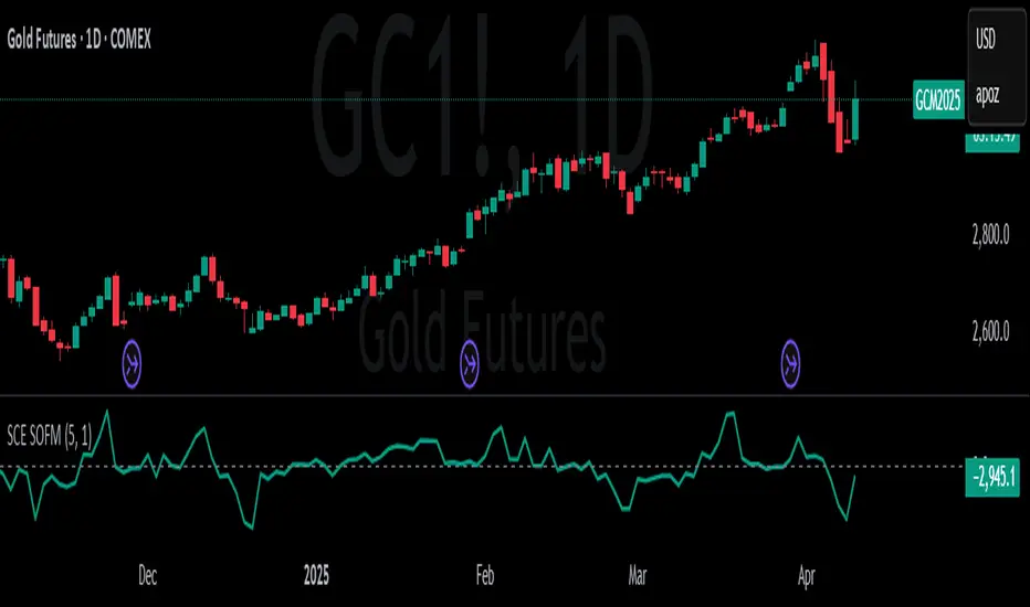
Stochastic Order Flow Momentum [ScorsoneEnterprises]This indicator implements a stochastic model of order flow using the Ornstein-Uhlenbeck (OU) process, combined with a Kalman filter to smooth momentum signals. It is designed to capture the dynamic momentum of volume delta, representing the net buying or selling pressure per bar, and highlight potential shifts in market direction. The volume delta data is sourced from TradingView’s built-in functionality:
www.tradingview.com
For a deeper dive into stochastic processes like the Ornstein-Uhlenbeck model in financial contexts, see these research articles: arxiv.org and arxiv.org
The SOFM tool aims to reveal the momentum and acceleration of order flow, modeled as a mean-reverting stochastic process. In markets, order flow often oscillates around a baseline, with bursts of buying or selling pressure that eventually fade—similar to how physical systems return to equilibrium. The OU process captures this behavior, while the Kalman filter refines the signal by filtering noise. Parameters theta (mean reversion rate), mu (mean level), and sigma (volatility) are estimated by minimizing a squared-error objective function using gradient descent, ensuring adaptability to real-time market conditions.
How It Works
The script combines a stochastic model with signal processing. Here’s a breakdown of the key components, including the OU equation and supporting functions.
// Ornstein-Uhlenbeck model for volume delta
ou_model(params, v_t, lkb) =>
theta = clamp(array.get(params, 0), 0.01, 1.0)
mu = clamp(array.get(params, 1), -100.0, 100.0)
sigma = clamp(array.get(params, 2), 0.01, 100.0)
error = 0.0
v_pred = array.new(lkb, 0.0)
array.set(v_pred, 0, array.get(v_t, 0))
for i = 1 to lkb - 1
v_prev = array.get(v_pred, i - 1)
v_curr = array.get(v_t, i)
// Discretized OU: v_t = v_{t-1} + theta * (mu - v_{t-1}) + sigma * noise
v_next = v_prev + theta * (mu - v_prev)
array.set(v_pred, i, v_next)
v_curr_clean = na(v_curr) ? 0 : v_curr
v_pred_clean = na(v_next) ? 0 : v_next
error := error + math.pow(v_curr_clean - v_pred_clean, 2)
error
The ou_model function implements a discretized Ornstein-Uhlenbeck process:
v_t = v_{t-1} + theta (mu - v_{t-1})
The model predicts volume delta (v_t) based on its previous value, adjusted by the mean-reverting term theta (mu - v_{t-1}), with sigma representing the volatility of random shocks (approximated in the Kalman filter).
Parameters Explained
The parameters theta, mu, and sigma represent distinct aspects of order flow dynamics:
Theta:
Definition: The mean reversion rate, controlling how quickly volume delta returns to its mean (mu). Constrained between 0.01 and 1.0 (e.g., clamp(array.get(params, 0), 0.01, 1.0)).
Interpretation: A higher theta indicates faster reversion (short-lived momentum), while a lower theta suggests persistent trends. Initial value is 0.1 in init_params.
In the Code: In ou_model, theta scales the pull toward \mu, influencing the predicted v_t.
Mu:
Definition: The long-term mean of volume delta, representing the equilibrium level of net buying/selling pressure. Constrained between -100.0 and 100.0 (e.g., clamp(array.get(params, 1), -100.0, 100.0)).
Interpretation: A positive mu suggests a bullish bias, while a negative mu indicates bearish pressure. Initial value is 0.0 in init_params.
In the Code: In ou_model, mu is the target level that v_t reverts to over time.
Sigma:
Definition: The volatility of volume delta, capturing the magnitude of random fluctuations. Constrained between 0.01 and 100.0 (e.g., clamp(array.get(params, 2), 0.01, 100.0)).
Interpretation: A higher sigma reflects choppier, noisier order flow, while a lower sigma indicates smoother behavior. Initial value is 0.1 in init_params.
In the Code: In the Kalman filter, sigma contributes to the error term, adjusting the smoothing process.
Summary:
theta: Speed of mean reversion (how fast momentum fades).
mu: Baseline order flow level (bullish or bearish bias).
sigma: Noise level (variability in order flow).
Other Parts of the Script
Clamp
A utility function to constrain parameters, preventing extreme values that could destabilize the model.
ObjectiveFunc
Defines the objective function (sum of squared errors) to minimize during parameter optimization. It compares the OU model’s predicted volume delta to observed data, returning a float to be minimized.
How It Works: Calls ou_model to generate predictions, computes the squared error for each timestep, and sums it. Used in optimization to assess parameter fit.
FiniteDifferenceGradient
Calculates the gradient of the objective function using finite differences. Think of it as finding the "slope" of the error surface for each parameter. It nudges each parameter (theta, mu, sigma) by a small amount (epsilon) and measures the change in error, returning an array of gradients.
Minimize
Performs gradient descent to optimize parameters. It iteratively adjusts theta, mu, and sigma by stepping down the "hill" of the error surface, using the gradients from FiniteDifferenceGradient. Stops when the gradient norm falls below a tolerance (0.001) or after 20 iterations.
Kalman Filter
Smooths the OU-modeled volume delta to extract momentum. It uses the optimized theta, mu, and sigma to predict the next state, then corrects it with observed data via the Kalman gain. The result is a cleaner momentum signal.
Applied
After initializing parameters (theta = 0.1, mu = 0.0, sigma = 0.1), the script optimizes them using volume delta data over the lookback period. The optimized parameters feed into the Kalman filter, producing a smoothed momentum array. The average momentum and its rate of change (acceleration) are calculated, though only momentum is plotted by default.
A rising momentum suggests increasing buying or selling pressure, while a flattening or reversing momentum indicates fading activity. Acceleration (not plotted here) could highlight rapid shifts.
Tool Examples
The SOFM indicator provides a dynamic view of order flow momentum, useful for spotting directional shifts or consolidation.
Low Time Frame Example: On a 5-minute chart of SEED_ALEXDRAYM_SHORTINTEREST2:NQ , a rising momentum above zero with a lookback of 5 might signal building buying pressure, while a drop below zero suggests selling dominance. Crossings of the zero line can mark transitions, though the focus is on trend strength rather than frequent crossovers.
High Time Frame Example: On a daily chart of NYSE:VST , a sustained positive momentum could confirm a bullish trend, while a sharp decline might warn of exhaustion. The mean-reverting nature of the OU process helps filter out noise on longer scales. It doesn’t make the most sense to use this on a high timeframe with what our data is.
Choppy Markets: When momentum oscillates near zero, it signals indecision or low conviction, helping traders avoid whipsaws. Larger deviations from zero suggest stronger directional moves to act on, this is on $STT.
Inputs
Lookback: Users can set the lookback period (default 5) to adjust the sensitivity of the OU model and Kalman filter. Shorter lookbacks react faster but may be noisier; longer lookbacks smooth more but lag slightly.
The user can also specify the timeframe they want the volume delta from. There is a default way to lower and expand the time frame based on the one we are looking at, but users have the flexibility.
No indicator is 100% accurate, and SOFM is no exception. It’s an estimation tool, blending stochastic modeling with signal processing to provide a leading view of order flow momentum. Use it alongside price action, support/resistance, and your own discretion for best results. I encourage comments and constructive criticism.
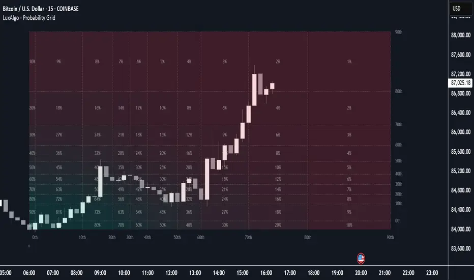
Probability Grid [LuxAlgo]The Probability Grid tool allows traders to see the probability of where and when the next reversal would occur, it displays a 10x10 grid and/or dashboard with the probability of the next reversal occurring beyond each cell or within each cell.
🔶 USAGE
By default, the tool displays deciles (percentiles from 0 to 90), users can enable, disable and modify each percentile, but two of them must always be enabled or the tool will display an error message alerting of it.
The use of the tool is quite simple, as shown in the chart above, the further the price moves on the grid, the higher the probability of a reversal.
In this case, the reversal took place on the cell with a probability of 9%, which means that there is a probability of 91% within the square defined by the last reversal and this cell.
🔹 Grid vs Dashboard
The tool can display a grid starting from the last reversal and/or a dashboard at three predefined locations, as shown in the chart above.
🔶 DETAILS
🔹 Raw Data vs Normalized Data
By default the tool displays the normalized data, this means that instead of using the raw data (price delta between reversals) it uses the returns between each reversal, this is useful to make an apples to apples comparison of all the data in the dataset.
This can be seen in the left side of the chart above (BTCUSD Daily chart) where normalize data is disabled, the percentiles from 0 to 40 overlap and are indistinguishable from each other because the tool uses the raw price delta over the entire bitcoin history, with normalize data enabled as we can see in the right side of the chart we can have a fair comparison of the data over the entire history.
🔹 Probability Beyond or Within Each Cell
Two different probability modes are available, the default mode is Probability Beyond Each Cell, the number displayed in each cell is the probability of the next reversal to be located in the area beyond the cell, for example, if the cell displays 20%, it means that in the area formed by the square starting from the last reversal and ending at the cell, there is an 80% probability and outside that square there is a 20% probability for the location of the next reversal.
The second probability mode is the probability within each cell, this outlines the chance that the next reversal will be within the cell, as we can see on the right chart above, when using deciles as percentiles (default settings), each cell has the same 1% probability for the 10x10 grid.
🔶 SETTINGS
Swing Length: The maximum length in bars used to identify a swing
Maximum Reversals: Maximum number of reversals included in calculations
Normalize Data: Use returns between swings instead of raw price
Probability: Choose between two different probability modes: beyond and inside each cell
Percentiles: Enable/disable each of the ten percentiles and select the percentile number and line style
🔹 Dashboard
Show Dashboard: Enable or disable the dashboard
Position: Choose dashboard location
Size: Choose dashboard size
🔹 Style
Show Grid: Enable or disable the grid
Size: Choose grid text size
Colors: Choose grid background colors
Show Marks: Enable/disable reversal markers
Sessions with Mausa session high/low tracker that draws flat, horizontal lines for Asia, London, and New York trading sessions. It updates those levels in real time during each session, locks them in once the session ends, and keeps them on the chart for context.
At a glance, you always know:
Where each session’s highs and lows were set
Which session produced them (ASIA, LDN, NY labels float cleanly above the highs)
When price is approaching or reacting to prior session levels
🔹 Use Cases:
• Key Levels – See where Asia, London, or NY set boundaries, and watch how price respects or rejects them
• Breakout Zones – Monitor when price breaks above/below session highs/lows
• Session Structure – Know instantly if a move happened during London or NY without squinting at the clock
• Backtesting – Keep historic session levels on the chart for reference — nothing gets deleted
• Confluence – Align these levels with support/resistance, fibs, or liquidity zones
Simple, visual, no distractions — just session structure at a glance.

Half Causal EstimatorOverview
The Half Causal Estimator is a specialized filtering method that provides responsive averages of market variables (volume, true range, or price change) with significantly reduced time delay compared to traditional moving averages. It employs a hybrid approach that leverages both historical data and time-of-day patterns to create a timely representation of market activity while maintaining smooth output.
Core Concept
Traditional moving averages suffer from time lag, which can delay signals and reduce their effectiveness for real-time decision making. The Half Causal Estimator addresses this limitation by using a non-causal filtering method that incorporates recent historical data (the causal component) alongside expected future behavior based on time-of-day patterns (the non-causal component).
This dual approach allows the filter to respond more quickly to changing market conditions while maintaining smoothness. The name "Half Causal" refers to this hybrid methodology—half of the data window comes from actual historical observations, while the other half is derived from time-of-day patterns observed over multiple days. By incorporating these "future" values from past patterns, the estimator can reduce the inherent lag present in traditional moving averages.
How It Works
The indicator operates through several coordinated steps. First, it stores and organizes market data by specific times of day (minutes/hours). Then it builds a profile of typical behavior for each time period. For calculations, it creates a filtering window where half consists of recent actual data and half consists of expected future values based on historical time-of-day patterns. Finally, it applies a kernel-based smoothing function to weight the values in this composite window.
This approach is particularly effective because market variables like volume, true range, and price changes tend to follow recognizable intraday patterns (they are positive values without DC components). By leveraging these patterns, the indicator doesn't try to predict future values in the traditional sense, but rather incorporates the average historical behavior at those future times into the current estimate.
The benefit of using this "average future data" approach is that it counteracts the lag inherent in traditional moving averages. In a standard moving average, recent price action is underweighted because older data points hold equal influence. By incorporating time-of-day averages for future periods, the Half Causal Estimator essentially shifts the center of the filter window closer to the current bar, resulting in more timely outputs while maintaining smoothing benefits.
Understanding Kernel Smoothing
At the heart of the Half Causal Estimator is kernel smoothing, a statistical technique that creates weighted averages where points closer to the center receive higher weights. This approach offers several advantages over simple moving averages. Unlike simple moving averages that weight all points equally, kernel smoothing applies a mathematically defined weight distribution. The weighting function helps minimize the impact of outliers and random fluctuations. Additionally, by adjusting the kernel width parameter, users can fine-tune the balance between responsiveness and smoothness.
The indicator supports three kernel types. The Gaussian kernel uses a bell-shaped distribution that weights central points heavily while still considering distant points. The Epanechnikov kernel employs a parabolic function that provides efficient noise reduction with a finite support range. The Triangular kernel applies a linear weighting that decreases uniformly from center to edges. These kernel functions provide the mathematical foundation for how the filter processes the combined window of past and "future" data points.
Applicable Data Sources
The indicator can be applied to three different data sources: volume (the trading volume of the security), true range (expressed as a percentage, measuring volatility), and change (the absolute percentage change from one closing price to the next).
Each of these variables shares the characteristic of being consistently positive and exhibiting cyclical intraday patterns, making them ideal candidates for this filtering approach.
Practical Applications
The Half Causal Estimator excels in scenarios where timely information is crucial. It helps in identifying volume climaxes or diminishing volume trends earlier than conventional indicators. It can detect changes in volatility patterns with reduced lag. The indicator is also useful for recognizing shifts in price momentum before they become obvious in price action, and providing smoother data for algorithmic trading systems that require reduced noise without sacrificing timeliness.
When volatility or volume spikes occur, conventional moving averages typically lag behind, potentially causing missed opportunities or delayed responses. The Half Causal Estimator produces signals that align more closely with actual market turns.
Technical Implementation
The implementation of the Half Causal Estimator involves several technical components working together. Data collection and organization is the first step—the indicator maintains a data structure that organizes market data by specific times of day. This creates a historical record of how volume, true range, or price change typically behaves at each minute/hour of the trading day.
For each calculation, the indicator constructs a composite window consisting of recent actual data points from the current session (the causal half) and historical averages for upcoming time periods from previous sessions (the non-causal half). The selected kernel function is then applied to this composite window, creating a weighted average where points closer to the center receive higher weights according to the mathematical properties of the chosen kernel. Finally, the kernel weights are normalized to ensure the output maintains proper scaling regardless of the kernel type or width parameter.
This framework enables the indicator to leverage the predictable time-of-day components in market data without trying to predict specific future values. Instead, it uses average historical patterns to reduce lag while maintaining the statistical benefits of smoothing techniques.
Configuration Options
The indicator provides several customization options. The data period setting determines the number of days of observations to store (0 uses all available data). Filter length controls the number of historical data points for the filter (total window size is length × 2 - 1). Filter width adjusts the width of the kernel function. Users can also select between Gaussian, Epanechnikov, and Triangular kernel functions, and customize visual settings such as colors and line width.
These parameters allow for fine-tuning the balance between responsiveness and smoothness based on individual trading preferences and the specific characteristics of the traded instrument.
Limitations
The indicator requires minute-based intraday timeframes, securities with volume data (when using volume as the source), and sufficient historical data to establish time-of-day patterns.
Conclusion
The Half Causal Estimator represents an innovative approach to technical analysis that addresses one of the fundamental limitations of traditional indicators: time lag. By incorporating time-of-day patterns into its calculations, it provides a more timely representation of market variables while maintaining the noise-reduction benefits of smoothing. This makes it a valuable tool for traders who need to make decisions based on real-time information about volume, volatility, or price changes.