Zig Zag + Fibonacci PROPlots ZigZag structure with optional Fibonacci retracement levels.
Helps identify recent highs/lows and possible support/resistance zones.
Customizable levels and alert on price cross.
Индикаторы ширины рынка

Hull MA with Support/Resistance📊 Combined Hull MA & Support/Resistance Indicator
🌟 Core Features Overview
This indicator integrates two powerful tools:
Hull Moving Average (Hull MA) - An optimized MA variant that reduces lag and closely follows price action.
Dynamic Support/Resistance System - Automatically identifies key price levels based on market structure.
Dual Advantage: Simultaneously identifies trends with Hull MA while pinpointing critical price zones for optimal entries.
⚙️ How It Works
Component Functionality Key Attributes Hull MA
- Trend identification
- Reversal signals via color changes - Low latency
- Color-coded (green/red) momentum
Support/Resistance - Key level detection
- Noise filtering via pivot points - Auto-adjusting
- Extended line visualization
📈 Practical Applications Trend Trading:
Buy when Hull MA turns green + price breaks Resistance
Sell when Hull MA turns red + price breaks Support
Breakout/Pullback Strategies:
Combine S/R breakouts with Hull MA slope for signal confirmation
Risk Management:
Place stop-loss orders beyond nearest S/R levels
⚡ Performance Optimization
Default Settings:
Hull MA: 16 periods (ideal for H1/D1 timeframes)
S/R: 1-bar pivot (short-term swing points)
Advanced Customization:
Increase Hull MA sensitivity by reducing periods
Widen S/R zones with Left/Right Bars >1
📌 Critical Notes
• Most effective in trending markets
• Recommended to combine with volume or RSI for confirmation
• Always backtest across multiple timeframes before live trading
💡 Pro Tip: Use Hull MA as primary trend filter - only trade when price retests S/R levels aligned with the MA's color.

Cumulative Delta Volume DivergenceCDV Divergence Indicator. Trading is about probabilities and no one indicator is going to give you a definite Buy/Sell signal. There are false positives. It can't tell you how high or low the price will go before it turns around. This is not financial advice. This is just a helpful addition to your toolbox :)

MOEX Sectors: % Above MA 50/100/200 (EMA/SMA)📊 Indicator Name:
MOEX Sector Breadth: % Above MA 50/100/200 (EMA/SMA)
📝 Description:
This indicator tracks market breadth across sector indices of the Moscow Exchange (MOEX). It calculates the percentage of sectors trading above selected moving averages (SMA or EMA) with user-defined periods (50, 100, or 200).
It provides a high-level view of market participation and internal strength, helping to identify broad trends, divergences, and potential reversals.
📦 Tracked MOEX Sector Indices:
mathematica
Copy
Edit
MOEXOG — Oil & Gas
MOEXCH — Chemicals
MOEXMM — Metals & Mining
MOEXTN — Transport
MOEXCN — Consumer
MOEXFN — Financials
MOEXTL — Telecom
MOEXEU — Utilities
MOEXIT — Information Technology
MOEXRE — Real Estate
📈 How to Use:
>50% above MA 200 → Bullish market regime
<50% above MA 200 → Weak breadth, caution advised
>90% above MA 50 → Market may be overbought
<10% above MA 200 → Market oversold, possible bottom
Combine with the IMOEX index to assess participation behind major moves
Use as a trend filter or divergence detector

IRUS: % stocks above SMA 50 / 100 / 200
📊 IRUS Breadth Indicators (MOEX Market Breadth)
This script shows market breadth conditions based on the percentage of stocks or sectors trading above selected moving averages (SMA or EMA) with customizable periods (50 / 100 / 200).
There are two modes available:
IRUS Ticker-Based Breadth
Calculates the % of liquid Russian stocks (IRUS group) trading above a selected MA.
Great for detailed breadth analysis based on individual stock participation.
Sector-Based Breadth
Calculates the % of major MOEX sector indices above their MAs.
A clean, high-level view of market strength across sectors.
Use these indicators to assess market health, detect divergences, and filter

Dskyz (DAFE) Aurora Divergence - Dskyz (DAFE) Aurora Divergence Indicator
Advanced Divergence Detection for Traders. Unleash the power of divergence trading with this cutting-edge indicator that combines price and volume analysis to spot high-probability reversal signals.
🧠 What Is It?
The Dskyz (DAFE) Aurora Divergence Indicator is designed to identify bullish and bearish divergences between the price trend and the On Balance Volume (OBV) trend. Divergence occurs when the price of an asset and a technical indicator (in this case, OBV) move in opposite directions, signaling a potential reversal. This indicator uses linear regression slopes to calculate the trends of both price and OBV over a specified lookback period, detecting when these two metrics are diverging. When a divergence is detected, it highlights potential reversal points with visually striking aurora bands, orbs, and labels, making it easy for traders to spot key signals.
⚙️ Inputs & How to Use Them
The indicator is highly customizable, with inputs grouped under "⚡ DAFE Aurora Settings" for clarity. Here’s how each input works:
Lookback Period: Determines how many bars are used to calculate the price and OBV slopes. Higher values detect longer-term trends (e.g., 20 for 1H charts), while lower values are more responsive to short-term movements.
Price Slope Threshold: Sets the minimum slope value for the price to be considered in an uptrend or downtrend. A value of 0 allows all slopes to be considered, while higher values filter for stronger trends.
OBV Slope Threshold: Similar to the price slope threshold but for OBV. Helps filter out weak volume trends.
Aurora Band Width: Adjusts the width of the visual bands that highlight divergence areas. Wider bands make the indicator more visible but may clutter the chart.
Divergence Sensitivity: Scales the strength of the divergence signals. Higher values make the indicator more sensitive to smaller divergences.
Minimum Strength: Filters out weak signals by only showing divergences above this strength level. A default of 0.3 is recommended for beginners.
Signal Cooldown (Bars): Prevents multiple signals from appearing too close together. Default is 5 bars, reducing chart clutter and helping traders focus on significant signals.
These inputs allow traders to fine-tune the indicator to match their trading style and timeframe.
🚀 What Makes It Unique?
This indicator stands out with its innovative features:
Price-Volume Divergence: Combines price trend (slope) and OBV trend for more reliable signals than price-only divergences.
Aurora Bands: Dynamic visual bands that highlight divergence zones, making it easier to spot potential reversals at a glance.
Interactive Dashboard: Displays real-time information on trend direction, volume flow, signal type, strength, and recommended actions (e.g., "Consider Buying" or "Consider Selling").
Signal Cooldown: Ensures only the most significant divergences are shown, reducing noise and improving usability.
Alerts: Built-in alerts for both bullish and bearish divergences, allowing traders to stay informed even when not actively monitoring the chart.
Beginner Guide: Explains the indicator’s visuals (e.g., aqua orbs for bullish signals, fuchsia orbs for bearish signals), making it accessible for new users.
🎯 Why It Works
The indicator’s effectiveness lies in its use of price-volume divergence, a well-established concept in technical analysis. When the price trend and OBV trend diverge, it often signals a potential reversal because the underlying volume support (or lack thereof) is not aligning with the price action. For example:
Bullish Divergence: Occurs when the price is making lower lows, but the OBV is making higher lows, indicating weakening selling pressure and potential upward reversal.
Bearish Divergence: Occurs when the price is making higher highs, but the OBV is making lower highs, suggesting weakening buying pressure and potential downward reversal.
The use of linear regression ensures smooth and accurate trend calculations over the specified lookback period. The divergence strength is then normalized and filtered based on user-defined thresholds, ensuring only high-quality signals are displayed. Additionally, the cooldown period prevents signal overload, allowing traders to focus on the most significant opportunities.
🧬 Indicator Recommendation
Best For: Traders looking to identify potential trend reversals in any market, especially those where volume data is reliable (e.g., stocks, futures, forex).
Timeframes: Suitable for all timeframes. Adjust the lookback period accordingly—smaller values for shorter timeframes (e.g., 1H), larger for longer ones (e.g., 4H or daily).
Pair With: Support and resistance levels, trend lines, other oscillators (e.g., RSI, MACD) for confirmation, and volume profile tools for deeper analysis.
Tips:
Look for divergences at key support/resistance levels for higher-probability setups.
Pay attention to signal strength; higher strength divergences are often more reliable.
Use the dashboard to quickly assess market conditions before entering a trade.
Set up alerts to catch divergences even when not actively watching the chart.
🧾 Credit & Acknowledgement
This indicator builds upon the classic concept of price-volume divergence, enhancing it with modern visualization techniques, advanced filtering, and user-friendly features. It is designed to provide traders with a powerful yet intuitive tool for spotting reversals.
📌 Final Thoughts
The Dskyz (DAFE) Aurora Divergence Indicator is more than just a divergence tool; it’s a comprehensive trading assistant that combines advanced calculations, intuitive visualizations, and actionable insights. Whether you’re a seasoned trader or just starting out, this indicator can help you spot high-probability reversal points with confidence.
Use it with discipline. Use it with clarity. Trade smarter.
**I will continue to release incredible strategies and indicators until I turn this into a brand or until someone offers me a contract.
-Dskyz

Moving average with different timeThis script allowing you to plot up to 6 different types of moving averages (MAs) on the chart, each with customizable parameters such as type, length, source, color, and timeframe. It also allows you to set different timeframes for each moving average.
Key Features:
Multiple Moving Averages: You can add up to 6 different moving averages to your chart.
Each MA can be one of the following types: SMA, EMA, SMMA (RMA), WMA, or VWMA.
Custom Timeframes: Each moving average can be applied to a specific timeframe, giving you flexibility to compare different periods (e.g., a 50-period moving average on the 1-hour chart and a 200-period moving average on the 4-hour chart).
Customizable Inputs:
Type: Choose between SMA, EMA, SMMA, WMA, or VWMA for each MA.
Source: You can select the price data source (e.g., close, open, high, low).
Length: Set the number of periods (length) for each moving average.
Color: Each moving average can be assigned a specific color.
Timeframe: Customize the timeframe for each moving average individually (e.g., MA1 on 15-minute, MA2 on 1-hour).
User Interface:
The script includes a data window display for each moving average, allowing you to control whether to show each MA and configure its settings directly from the settings menu.
Flexible Use:
Toggle individual moving averages on and off with the show checkbox for each MA.
Customize each MA's parameters without affecting others.
Parameters:
MA Type: You can choose between different moving averages (SMA, EMA, etc.).
Source: Price data used for calculating the moving average (e.g., close, open, etc.).
Length: Defines the period (number of bars) for each moving average.
Color: Change the line color for each moving average for better visualization.
Timeframe: Set a different timeframe for each moving average (e.g., 1-day MA vs. 1-week MA).
Example Use Case:
You might use this indicator to track short-term, medium-term, and long-term trends by adding multiple MAs with different lengths and timeframes. For example:
MA1 (20-period) might be an SMA on a 1-hour chart.
MA2 (50-period) might be an EMA on a 4-hour chart.
MA3 (100-period) might be a WMA on a daily chart.
This setup allows you to visually track the market's behavior across different timeframes and better identify trends, crossovers, and other patterns.
How to Customize:
Show/Hide MAs: Enable or disable each moving average from the input menu.
Modify Parameters: Change the MA type, source, length, and color for each individual moving average.
Timeframes: Set different timeframes for each moving average for more detailed analysis.
With this Moving Average Ribbon, you get a versatile and visually rich tool to aid in technical analysis.

Change % - NQ / ES / YM Funded Futures Risk Manager – NQ / ES / YM
🎯 Purpose
This tool is designed for funded futures traders who need to comply with daily risk rules from Topstep, Apex, and similar programs. It tracks the real-time daily % price change in major U.S. equity index futures: Nasdaq (NQ), S&P 500 (ES), and Dow Jones (YM).
⚠️ Why It Matters
Most funded trading programs prohibit trading when the market is within 2% of CME’s daily price limits. This script provides a clear, real-time visual warning to help avoid account violations or disqualification.
🧠 What It Does
Detects the instrument (NQ1!, ES1!, YM1!, and front-month contracts like NQM2025)
Calculates % change from the daily open
Simulates CME’s ±7% daily limit bands
Displays a floating panel with current change in %
Shows a warning if price is within the restricted last 2%
Optionally triggers a visual or sound alert
🔍 Why It’s Different
This is not a predictive or technical analysis tool.
It’s a real-time compliance assistant designed to protect your funded account during volatile sessions.
No complex logic, just clear visual safety for serious traders.
🧭 How To Use It
Add the script to your chart
Use it on NQ1!, ES1!, or YM1! (or M2025 contracts)
The panel shows live price change % from today’s open
When price enters the last 2% of CME’s limit, a warning appears
Avoid entering trades during these times to stay compliant
🖼️ Recommended Chart Setup
✔️ Only this script applied
✔️ Show ticker, timeframe, and the floating panel
✔️ Clean background (no extra drawings or indicators)
✔️ Use on a volatile day for better demonstration (e.g. -2% day)
✅ Fully compliant with TradingView’s script publishing rules.
✅ Focused on risk awareness and rule enforcement.
✅ Supports real-world funded traders.

[blackcat] L2 Ehlers Autocorrelation Indicator V2OVERVIEW
The Ehlers Autocorrelation Indicator is a technical analysis tool developed by John F. Ehlers that measures the correlation between price data and its lagged versions to identify potential market cycles and reversals.
BACKGROUND
Originally introduced in Ehlers' "Cycle Analytics for Traders" (2013), this indicator leverages autocorrelation principles to detect patterns in market data that deviate from random noise or perfect sine waves.
FEATURES
• Calculates Pearson correlation coefficients for lags from 0 to 60 bars
• Visualizes correlations using colored bars ranging from red (negative correlation) to yellow (positive correlation)
• Provides minimum averaging option through AvgLength input parameter
• Displays sharp reversal signals at price turning points
• Shows variations in bar thickness and count over time
HOW TO USE
Add the indicator to your chart
Adjust the AvgLength input as needed:
• Set to 0 for no averaging
• Increase value for smoother results
Interpret the colored bars:
• Red: Negative correlation
• Yellow: Positive correlation
• Sharp transitions indicate potential reversal points
LIMITATIONS
• Requires sufficient historical data for accurate calculations
• Performance may vary across different market conditions
• Results depend on proper parameter settings
NOTES
• The indicator uses highpass filtering and super smoother filtering techniques
• Color intensity varies based on correlation strength
• Multiple lag periods are displayed simultaneously for comprehensive analysis
THANKS
This implementation is based on Ehlers' original work and has been adapted for TradingView's Pine Script platform.

Smart Money Visual Suite [ALFANAR_Q8]📈 Smart Money Visual Suite
🔒 Read-only visual indicator – no entry/exit signals, purely for Smart Money concept analysis.
Features:
🔄 CHoCH and BOS for market structure shifts
🎯 Inducement and Sweeps to highlight liquidity targets
🔁 Zigzag to clarify price action waves
💡 RSI Divergence to detect potential reversals
🟩 Demand Zones (green) & 🟥 Supply Zones (red), designed for dark theme charts
🧠 Built on Smart Money principles – perfect for traders seeking clean visual structure and liquidity analysis.
🚫 No buy/sell signals – this tool is for visual market structure interpretation only.

Moving Averages & RSIThis TradingView Pine Script plots multiple moving averages (EMAs, SMAs) and multi-timeframe RSI values for trend analysis.
It includes a regime filter based on sector and index trends (e.g., SPX, XLF, XLK) to highlight market conditions.
Bullish and bearish RSI divergences are detected and visually flagged on the chart.
Several UI tables display RSI values, sector info, market trend status, and share float, with optional watermark labeling.

Average Body RangeThe Average Body Range (ABR) indicator calculates the average size of a candle's real body over a specified period. Unlike the traditional Average Daily Range (ADR), which measures the full range from high to low, the ABR focuses solely on the absolute difference between the open and close of each bar. This provides insight into market momentum and trading activity by reflecting how much price is actually moving from open to close , not just in total.
This indicator is especially useful for identifying:
Periods of strong directional movement (larger body sizes)
Low-volatility or indecisive markets (smaller body sizes)
Changes in trend conviction or momentum
Customization:
Length: Number of bars used to compute the average (default: 14)
Use ABR to enhance your understanding of price behavior and better time entries or exits based on market strength.

FT-RSISummary of the Custom RSI Indicator Script (For Futu Niuniu Platform):
This Pine Script code implements a triple-period RSI indicator with horizontal reference lines (70, 50, 30) for technical analysis on the Futu Niuniu trading platform.
Key Features:
Multi-period RSI Calculation:
Computes three RSI values using 9, 14, and 22-period lengths to capture short-term, standard, and smoothed momentum signals.
Utilizes the Relative Moving Average (RMA) method for RSI calculation (ta.rma function).
Horizontal Reference Bands:
Upper Band (70): Red dotted line (semi-transparent) to identify overbought conditions.
Middle Band (50): Green dotted line as the neutral equilibrium level.
Lower Band (30): Blue dotted line (semi-transparent) to highlight oversold zones.
Visual Customization:
Distinct colors for each RSI line:
RSI (9): Orange (#F79A00)
RSI (14): Green (#49B50D)
RSI (22): Blue (#5188FF)
All lines have a thickness of 2 pixels for clear visibility.
Platform Compatibility:
This script is designed for Futu Niuniu’s charting system, leveraging Pine Script syntax adaptations supported by the platform. The horizontal bands and multi-period RSI logic help traders analyze trend strength and potential reversal points efficiently.
Note: Ensure Futu Niuniu’s scripting environment supports ta.rma and hline functions for proper execution.

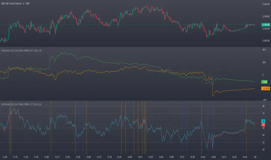
OBV & AD Oscillators with Dual Smoothing OptionsOn Balance Volume and Accumulation/Distribution
Overlaid into 1 and then some,
Now it is an oscillator!
3 customizable moving average types
- Ehlers Deviation Scaled Moving Average
- Volatility Dynamic Moving Average
- Simple Moving Average
Each with customizable periods
And with the ability to overlay a second set too
Default Settings have a longer period MA of 377 using Ehlers DSMA to better capture the standard view of OBV and A/D.
An extra overlay of a shorter period using a Volatility DMA uses Average True Range with its own custom settings, seeks to act more as an RSI
Mongoose Yield Spread Dashboard v5 – Labeled, Alerted, ReadableCurveGuard: Mongoose Edition
Track the macro tide before it turns.
This tool visualizes the three most-watched U.S. Treasury yield curve spreads:
2s10s (10Y - 2Y)
5s30s (30Y - 5Y)
3M10Y (10Y - 3M)
Each spread is plotted with dynamic color logic, inversion alerts, and floating labels. Background shading highlights historical inversion zones to help spot macro regime shifts in real time.
✅ Alert-ready
✅ Dark mode optimized
✅ Floating labels
✅ Clean layout for fast macro insight
📌 For educational and informational purposes only.
This script does not provide financial advice or trade recommendations.

DI+/- Cross Strategy with ATR SL and 2% TPDI+/- Cross Strategy with ATR Stop Loss and 2% Take Profit
📝 Script Description for Publishing:
This strategy is based on the directional movement of the market using the Average Directional Index (ADX) components — DI+ and DI- — to generate entry signals, with clearly defined risk and reward targets using ATR-based Stop Loss and Fixed Percentage Take Profit.
🔍 How it works:
Buy Signal: When DI+ crosses above 40, signaling strong bullish momentum.
Sell Signal: When DI- crosses above 40, indicating strong bearish momentum.
Stop Loss: Dynamically calculated using ATR × 1.5, to account for market volatility.
Take Profit: Fixed at 2% above/below the entry price, for consistent reward targeting.
🧠 Why it’s useful:
Combines momentum breakout logic with volatility-based risk management.
Works well on trending assets, especially when combined with higher timeframe filters.
Clean BUY and SELL visual labels make it easy to interpret and backtest.
✅ Tips for Use:
Use on assets with clear trends (e.g., major forex pairs, trending stocks, crypto).
Best on 30m – 4H timeframes, but can be customized.
Consider combining with other filters (e.g., EMA trend direction or Bollinger Bands) for even better accuracy.

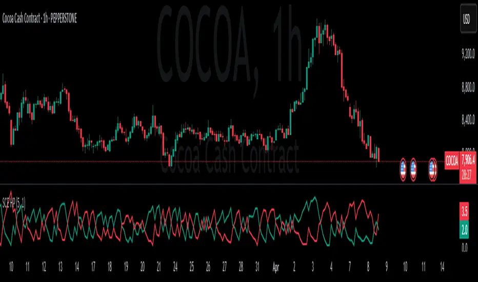
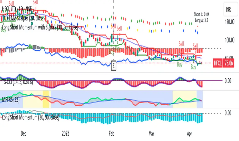
Long Short Momentum with Signals
Long and Short momentum
WHEN SHORT MOMENTUM CHANGES 2.0 POINTS and long term changes 5 points on day basis write A for Bullish and B for Bearish on Main Price chart
WHEN SHORT MOMENTUM CHANGES .30 per hour POINTS and long term changes 1 points on 1 hour basis. Put a green dot for Bull and red for bear in short term and for long termRespectively on price chart
PMO + Daily SMA(55)PMO + Daily SMA(55)
This script plots the Price Momentum Oscillator (PMO) using the classic DecisionPoint methodology, along with its signal line and the 55-period Simple Moving Average (SMA) of the daily PMO.
PMO is a smoothed momentum indicator that measures the rate of change and helps identify trend direction and strength. The signal line is an EMA of the PMO, commonly used for crossover signals.
The 55-period SMA of the daily PMO is added as a longer-term trend filter. It remains based on daily data, even when applied to intraday charts, making it useful for aligning lower timeframe trades with higher timeframe momentum.
Ideal for swing and position traders looking to combine short-term momentum with broader trend context.

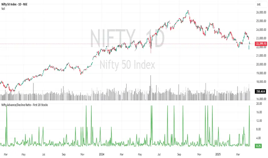
Nifty Advance/Decline Ratio - First 20 StocksNifty 20 Advance/Decline Ratio Indicator
This Pine Script tracks the Advance/Decline Ratio of the top 20 Nifty stocks (by weightage as of March 31, 2025). It helps gauge the market's strength by comparing the number of advancing vs. declining stocks among major Nifty heavyweights. The script calculates and plots the ratio, with a reference line at 1 (neutral point). This indicator resets daily and provides insights into overall market trends based on the performance of the top Nifty stocks.
Key Features:
Tracks advance/decline movements of top 20 Nifty stocks.
Plots the Advance/Decline Ratio on the chart.
Resets daily for fresh analysis.
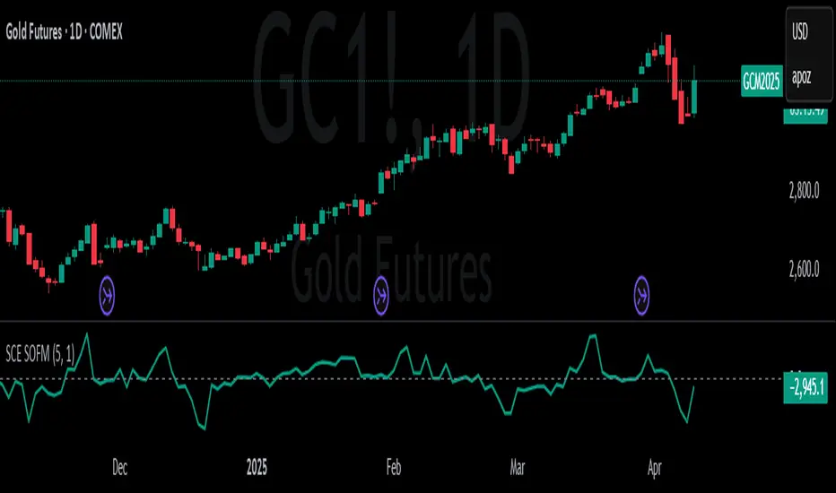
Stochastic Order Flow Momentum [ScorsoneEnterprises]This indicator implements a stochastic model of order flow using the Ornstein-Uhlenbeck (OU) process, combined with a Kalman filter to smooth momentum signals. It is designed to capture the dynamic momentum of volume delta, representing the net buying or selling pressure per bar, and highlight potential shifts in market direction. The volume delta data is sourced from TradingView’s built-in functionality:
www.tradingview.com
For a deeper dive into stochastic processes like the Ornstein-Uhlenbeck model in financial contexts, see these research articles: arxiv.org and arxiv.org
The SOFM tool aims to reveal the momentum and acceleration of order flow, modeled as a mean-reverting stochastic process. In markets, order flow often oscillates around a baseline, with bursts of buying or selling pressure that eventually fade—similar to how physical systems return to equilibrium. The OU process captures this behavior, while the Kalman filter refines the signal by filtering noise. Parameters theta (mean reversion rate), mu (mean level), and sigma (volatility) are estimated by minimizing a squared-error objective function using gradient descent, ensuring adaptability to real-time market conditions.
How It Works
The script combines a stochastic model with signal processing. Here’s a breakdown of the key components, including the OU equation and supporting functions.
// Ornstein-Uhlenbeck model for volume delta
ou_model(params, v_t, lkb) =>
theta = clamp(array.get(params, 0), 0.01, 1.0)
mu = clamp(array.get(params, 1), -100.0, 100.0)
sigma = clamp(array.get(params, 2), 0.01, 100.0)
error = 0.0
v_pred = array.new(lkb, 0.0)
array.set(v_pred, 0, array.get(v_t, 0))
for i = 1 to lkb - 1
v_prev = array.get(v_pred, i - 1)
v_curr = array.get(v_t, i)
// Discretized OU: v_t = v_{t-1} + theta * (mu - v_{t-1}) + sigma * noise
v_next = v_prev + theta * (mu - v_prev)
array.set(v_pred, i, v_next)
v_curr_clean = na(v_curr) ? 0 : v_curr
v_pred_clean = na(v_next) ? 0 : v_next
error := error + math.pow(v_curr_clean - v_pred_clean, 2)
error
The ou_model function implements a discretized Ornstein-Uhlenbeck process:
v_t = v_{t-1} + theta (mu - v_{t-1})
The model predicts volume delta (v_t) based on its previous value, adjusted by the mean-reverting term theta (mu - v_{t-1}), with sigma representing the volatility of random shocks (approximated in the Kalman filter).
Parameters Explained
The parameters theta, mu, and sigma represent distinct aspects of order flow dynamics:
Theta:
Definition: The mean reversion rate, controlling how quickly volume delta returns to its mean (mu). Constrained between 0.01 and 1.0 (e.g., clamp(array.get(params, 0), 0.01, 1.0)).
Interpretation: A higher theta indicates faster reversion (short-lived momentum), while a lower theta suggests persistent trends. Initial value is 0.1 in init_params.
In the Code: In ou_model, theta scales the pull toward \mu, influencing the predicted v_t.
Mu:
Definition: The long-term mean of volume delta, representing the equilibrium level of net buying/selling pressure. Constrained between -100.0 and 100.0 (e.g., clamp(array.get(params, 1), -100.0, 100.0)).
Interpretation: A positive mu suggests a bullish bias, while a negative mu indicates bearish pressure. Initial value is 0.0 in init_params.
In the Code: In ou_model, mu is the target level that v_t reverts to over time.
Sigma:
Definition: The volatility of volume delta, capturing the magnitude of random fluctuations. Constrained between 0.01 and 100.0 (e.g., clamp(array.get(params, 2), 0.01, 100.0)).
Interpretation: A higher sigma reflects choppier, noisier order flow, while a lower sigma indicates smoother behavior. Initial value is 0.1 in init_params.
In the Code: In the Kalman filter, sigma contributes to the error term, adjusting the smoothing process.
Summary:
theta: Speed of mean reversion (how fast momentum fades).
mu: Baseline order flow level (bullish or bearish bias).
sigma: Noise level (variability in order flow).
Other Parts of the Script
Clamp
A utility function to constrain parameters, preventing extreme values that could destabilize the model.
ObjectiveFunc
Defines the objective function (sum of squared errors) to minimize during parameter optimization. It compares the OU model’s predicted volume delta to observed data, returning a float to be minimized.
How It Works: Calls ou_model to generate predictions, computes the squared error for each timestep, and sums it. Used in optimization to assess parameter fit.
FiniteDifferenceGradient
Calculates the gradient of the objective function using finite differences. Think of it as finding the "slope" of the error surface for each parameter. It nudges each parameter (theta, mu, sigma) by a small amount (epsilon) and measures the change in error, returning an array of gradients.
Minimize
Performs gradient descent to optimize parameters. It iteratively adjusts theta, mu, and sigma by stepping down the "hill" of the error surface, using the gradients from FiniteDifferenceGradient. Stops when the gradient norm falls below a tolerance (0.001) or after 20 iterations.
Kalman Filter
Smooths the OU-modeled volume delta to extract momentum. It uses the optimized theta, mu, and sigma to predict the next state, then corrects it with observed data via the Kalman gain. The result is a cleaner momentum signal.
Applied
After initializing parameters (theta = 0.1, mu = 0.0, sigma = 0.1), the script optimizes them using volume delta data over the lookback period. The optimized parameters feed into the Kalman filter, producing a smoothed momentum array. The average momentum and its rate of change (acceleration) are calculated, though only momentum is plotted by default.
A rising momentum suggests increasing buying or selling pressure, while a flattening or reversing momentum indicates fading activity. Acceleration (not plotted here) could highlight rapid shifts.
Tool Examples
The SOFM indicator provides a dynamic view of order flow momentum, useful for spotting directional shifts or consolidation.
Low Time Frame Example: On a 5-minute chart of SEED_ALEXDRAYM_SHORTINTEREST2:NQ , a rising momentum above zero with a lookback of 5 might signal building buying pressure, while a drop below zero suggests selling dominance. Crossings of the zero line can mark transitions, though the focus is on trend strength rather than frequent crossovers.
High Time Frame Example: On a daily chart of NYSE:VST , a sustained positive momentum could confirm a bullish trend, while a sharp decline might warn of exhaustion. The mean-reverting nature of the OU process helps filter out noise on longer scales. It doesn’t make the most sense to use this on a high timeframe with what our data is.
Choppy Markets: When momentum oscillates near zero, it signals indecision or low conviction, helping traders avoid whipsaws. Larger deviations from zero suggest stronger directional moves to act on, this is on $STT.
Inputs
Lookback: Users can set the lookback period (default 5) to adjust the sensitivity of the OU model and Kalman filter. Shorter lookbacks react faster but may be noisier; longer lookbacks smooth more but lag slightly.
The user can also specify the timeframe they want the volume delta from. There is a default way to lower and expand the time frame based on the one we are looking at, but users have the flexibility.
No indicator is 100% accurate, and SOFM is no exception. It’s an estimation tool, blending stochastic modeling with signal processing to provide a leading view of order flow momentum. Use it alongside price action, support/resistance, and your own discretion for best results. I encourage comments and constructive criticism.
Trend Confirmation StrategyComprehensive Trend Confirmation System
Indicator Features (Professional Description):
Comprehensive Trend Confirmation System is a versatile indicator meticulously designed to identify and confirm trend-based trading opportunities with exceptional efficiency. By seamlessly integrating analysis from a suite of leading technical tools, it aims to provide superior accuracy and reliability for informed trading decisions.
Key Features:
Intelligent Trend Identification: A robust trend analysis system that considers:
Adjustable Moving Averages: Utilizes three customizable moving average periods (fast, medium, slow) with user-selectable lengths and types (SMA, EMA, WMA, VWMA) to accurately determine the prevailing trend across different timeframes.
In-depth Price Action Analysis: Examines the formation of Higher Highs/Higher Lows (uptrend) and Lower Highs/Lower Lows (downtrend) to validate price direction.
Average Directional Index (ADX) with Adjustable Threshold: Measures the strength of a trend and employs the comparison between +DI and -DI to pinpoint the dominant momentum, featuring a customizable threshold to filter out weak signals.
Multi-Factor Signal Confirmation System: Enhances the reliability of trading signals through verification from four distinct confirmation tools:
Volume Analysis with Average Reference: Assesses whether trading volume supports price movements by comparing it to historical averages.
Relative Strength Index (RSI) with Reference Levels: Measures price momentum and identifies overbought/oversold conditions to confirm trend strength.
Moving Average Convergence Divergence (MACD) Divergence and Crossovers: Detects shifts in momentum and potential trend changes through the relationship between the MACD line and the Signal line.
Stochastic Oscillator with Reference Levels: Measures the current price's position relative to its historical range to evaluate overbought/oversold conditions and potential reversal opportunities.
Intelligent Signal Generation Logic:
Buy Signal: Triggered when a strong uptrend is identified (meeting defined criteria) and confirmed by at least three out of the four confirmation tools.
Sell Signal: Triggered when a strong downtrend is identified (meeting defined criteria) and confirmed by at least three out of the four confirmation tools.
User-Friendly Visualizations:
Moving Averages (MA): Displays three MA lines on the chart with user-configurable colors (default: fast-blue, medium-orange, slow-red) for easy visual trend analysis.
Clear Buy and Sell Signal Symbols: Presents distinct green upward-pointing triangles for buy signals and red downward-pointing triangles for sell signals at the corresponding candlestick.
Dynamic Candlestick Color Coding: Candlesticks are dynamically colored green upon a buy signal and red upon a sell signal for quick identification of trading opportunities.
Highly Customizable Parameters: Users have extensive control over the indicator's parameters, including:
Lengths and types of Moving Averages.
Length and Threshold of the ADX.
Length of the RSI.
Parameters for the MACD (Fast Length, Slow Length, Signal Length).
Parameters for the Stochastic Oscillator (%K Length, %D Length, Smoothing).
Ideal For:
Traders seeking a robust tool to accurately identify and confirm market trends.
Individuals aiming to reduce false signals and enhance the precision of their trading decisions.
Traders employing trend-following strategies in markets with clear directional movement.
Important Note:
While Comprehensive Trend Confirmation System is engineered to improve trading accuracy, no indicator can guarantee 100% profitable trades. Users are advised to utilize this indicator in conjunction with relevant fundamental analysis and sound risk management practices for optimal trading outcomes.

Order Flow Hawkes Process [ScorsoneEnterprises]This indicator is an implementation of the Hawkes Process. This tool is designed to show the excitability of the different sides of volume, it is an estimation of bid and ask size per bar. The code for the volume delta is from www.tradingview.com
Here’s a link to a more sophisticated research article about Hawkes Process than this post arxiv.org
This tool is designed to show how excitable the different sides are. Excitability refers to how likely that side is to get more activity. Alan Hawkes made Hawkes Process for seismology. A big earthquake happens, lots of little ones follow until it returns to normal. Same for financial markets, big orders come in, causing a lot of little orders to come. Alpha, Beta, and Lambda parameters are estimated by minimizing a negative log likelihood function.
How it works
There are a few components to this script, so we’ll go into the equation and then the other functions used in this script.
hawkes_process(params, events, lkb) =>
alpha = clamp(array.get(params, 0), 0.01, 1.0)
beta = clamp(array.get(params, 1), 0.1, 10.0)
lambda_0 = clamp(array.get(params, 2), 0.01, 0.3)
intensity = array.new_float(lkb, 0.0)
events_array = array.new_float(lkb, 0.0)
for i = 0 to lkb - 1
array.set(events_array, i, array.get(events, i))
for i = 0 to lkb - 1
sum_decay = 0.0
current_event = array.get(events_array, i)
for j = 0 to i - 1
time_diff = i - j
past_event = array.get(events_array, j)
decay = math.exp(-beta * time_diff)
past_event_val = na(past_event) ? 0 : past_event
sum_decay := sum_decay + (past_event_val * decay)
array.set(intensity, i, lambda_0 + alpha * sum_decay)
intensity
The parameters alpha, beta, and lambda all represent a different real thing.
Alpha (α):
Definition: Alpha represents the excitation factor or the magnitude of the influence that past events have on the future intensity of the process. In simpler terms, it measures how much each event "excites" or triggers additional events. It is constrained between 0.01 and 1.0 (e.g., clamp(array.get(params, 0), 0.01, 1.0)). A higher alpha means past events have a stronger influence on increasing the intensity (likelihood) of future events. Initial value is set to 0.1 in init_params. In the hawkes_process function, alpha scales the contribution of past events to the current intensity via the term alpha * sum_decay.
Beta (β):
Definition: Beta controls the rate of exponential decay of the influence of past events over time. It determines how quickly the effect of a past event fades away. It is constrained between 0.1 and 10.0 (e.g., clamp(array.get(params, 1), 0.1, 10.0)). A higher beta means the influence of past events decays faster, while a lower beta means the influence lingers longer. Initial value is set to 0.1 in init_params. In the hawkes_process function, beta appears in the decay term math.exp(-beta * time_diff), which reduces the impact of past events as the time difference (time_diff) increases.
Lambda_0 (λ₀):
Definition: Lambda_0 is the baseline intensity of the process, representing the rate at which events occur in the absence of any excitation from past events. It’s the "background" rate of the process. It is constrained between 0.01 and 0.3 .A higher lambda_0 means a higher natural frequency of events, even without the influence of past events. Initial value is set to 0.1 in init_params. In the hawkes_process function, lambda_0 sets the minimum intensity level, to which the excitation term (alpha * sum_decay) is added: lambda_0 + alpha * sum_decay
Alpha (α): Strength of event excitation (how much past events boost future events).
Beta (β): Rate of decay of past event influence (how fast the effect fades).
Lambda_0 (λ₀): Baseline event rate (background intensity without excitation).
Other parts of the script.
Clamp
The clamping function is a simple way to make sure parameters don’t grow or shrink too much.
ObjectiveFunction
This function defines the objective function (negative log-likelihood) to minimize during parameter optimization.It returns a float representing the negative log-likelihood (to be minimized).
How It Works:
Calls hawkes_process to compute the intensity array based on current parameters.Iterates over the lookback period:lambda_t: Intensity at time i.event: Event magnitude at time i.Handles na values by replacing them with 0.Computes log-likelihood: event_clean * math.log(math.max(lambda_t_clean, 0.001)) - lambda_t_clean.Ensures lambda_t_clean is at least 0.001 to avoid log(0).Accumulates into log_likelihood.Returns -log_likelihood (negative because the goal is to minimize, not maximize).
It is used in the optimization process to evaluate how well the parameters fit the observed event data.
Finite Difference Gradient:
This function calculates the gradient of the objective function we spoke about. The gradient is like a directional derivative. Which is like the direction of the rate of change. Which is like the direction of the slope of a hill, we can go up or down a hill. It nudges around the parameter, and calculates the derivative of the parameter. The array of these nudged around parameters is what is returned after they are optimized.
Minimize:
This is the function that actually has the loop and calls the Finite Difference Gradient each time. Here is where the minimizing happens, how we go down the hill. If we are below a tolerance, we are at the bottom of the hill.
Applied
After an initial guess the parameters are optimized with a mix of bid and ask levels to prevent some over-fitting for each side while keeping some efficiency. We initialize two different arrays to store the bid and ask sizes. After we optimize the parameters we clamp them for the calculations. We then get the array of intensities from the Hawkes Process of bid and ask and plot them both. When the bids are greater than the ask it represents a bullish scenario where there are likely to be more buy than sell orders, pushing up price.
Tool examples:
The idea is that when the bid side is more excitable it is more likely to see a bullish reaction, when the ask is we see a bearish reaction.
We see that there are a lot of crossovers, and I picked two specific spots. The idea of this isn’t to spot crossovers but avoid chop. The values are either close together or far apart. When they are far, it is a classification for us to look for our own opportunities in, when they are close, it signals the market can’t pick a direction just yet.
The value works just as well on a higher timeframe as on a lower one. Hawkes Process is an estimate, so there is a leading value aspect of it.
The value works on equities as well, here is NASDAQ:TSLA on a lower time frame with a lookback of 5.
Inputs
Users can enter the lookback value and timeframe.
No tool is perfect, the Hawkes Process value is also not perfect and should not be followed blindly. It is good to use any tool along with discretion and price action.